Devy Ratnasari
Government bonds buyer predictions
The analysis is conducted to predict how much government bonds the company has to order based on the users behaviour. The dataset is sourced from Indonesia Fintech StartUp between August and October 2021.
Users information
This dataset contains:- user_id - User's identity
- registration_import_datetime - Date of user registered
- user_gender - Gender of the user
- user_age - Age of the user
- user_occupation - Occupation of the user
- user_income_range - Range income of the user
- referral_code_used - If the user using referral code during registration or not
- user_income_source - The source of income from the user
| user_id | registration_import_datetime | user_gender | user_age | user_occupation | user_income_range | referral_code_used | user_income_source | |
|---|---|---|---|---|---|---|---|---|
| 0 | 162882 | 2021-09-17 | Female | 51 | Swasta | > Rp 500 Juta - 1 Miliar | NaN | Gaji |
| 1 | 3485491 | 2021-10-09 | Female | 55 | Others | > Rp 50 Juta - 100 Juta | NaN | Gaji |
| 2 | 1071649 | 2021-10-08 | Male | 50 | Swasta | Rp 10 Juta - 50 Juta | NaN | Gaji |
| 3 | 3816789 | 2021-08-12 | Female | 53 | IRT | > Rp 50 Juta - 100 Juta | NaN | Gaji |
| 4 | 3802293 | 2021-08-15 | Female | 47 | PNS | > Rp 500 Juta - 1 Miliar | used referral | Gaji |
User's daily transaction
This dataset contains:- user_id - Id of user, it's same with the user_id from dataset 1
- date - Transaction date
- Saham_AUM - AUM (../assets Under Management) of equity mutual fund held by client to date
- Saham_invested_amount - The total price paid by client to buy equity mutual fund to date.
- Saham_transaction_amount - Total value of transaction to buy (if positive) or sell (if negative) equity mutual fund on the date.
- Pasar_Uang_AUM - AUM of money market mutual fund held by client to date
- Pasar_Uang_invested_amount - The total price paid by client to buy money market mutual fund to date
- Pasar_Uang_transaction_amount - Total value of transaction to buy (if positive) or sell (if negative) money market mutual fund on the date.
- Pendapatan_Tetap_AUM - AUM of fixed income mutual fund held by client to date
- Pendapatan_Tetap_invested_amount - The total price paid by client to buy fixed income mutual fund to date
- Pendapatan_Tetap_transaction_amount - Total value of transaction to buy (if positive) or sell (if negative) fixed income mutual fund on the date.
- Campuran_AUM - AUM of mixed mutual fund held by client to date
- Campuran_invested_amount - The total price paid by client to buy mixed mutual fund to date
- Campuran_transaction_amount - Total value of the transaction to buy (if positive) or sell (if negative) mixed mutual fund on the date.
| user_id | trans_date | Saham_AUM | Saham_invested_amount | Saham_transaction_amount | Pasar_Uang_AUM | Pasar_Uang_invested_amount | Pasar_Uang_transaction_amount | Pendapatan_Tetap_AUM | Pendapatan_Tetap_invested_amount | Pendapatan_Tetap_transaction_amount | Campuran_AUM | Campuran_invested_amount | Campuran_transaction_amount | |
|---|---|---|---|---|---|---|---|---|---|---|---|---|---|---|
| 0 | 50701 | 2021-08-30 | 0.0 | 0.0 | 0.0 | 0.0 | 0.0 | 0.0 | 0.0 | 0.0 | 0.0 | 10132277.0 | 10000000.0 | 0.0 |
| 1 | 50701 | 2021-08-31 | 0.0 | 0.0 | 0.0 | 0.0 | 0.0 | 0.0 | 0.0 | 0.0 | 0.0 | 10206945.0 | 10000000.0 | 0.0 |
| 2 | 50701 | 2021-09-01 | 0.0 | 0.0 | 0.0 | 0.0 | 0.0 | 0.0 | 0.0 | 0.0 | 0.0 | 9956556.0 | 10000000.0 | 0.0 |
| 3 | 50701 | 2021-09-02 | 0.0 | 0.0 | 0.0 | 0.0 | 0.0 | 0.0 | 0.0 | 0.0 | 0.0 | 9914858.0 | 10000000.0 | 0.0 |
| 4 | 50701 | 2021-09-03 | 0.0 | 0.0 | 0.0 | 0.0 | 0.0 | 0.0 | 0.0 | 0.0 | 0.0 | 10016360.0 | 10000000.0 | 0.0 |
Bonds history purchase
This dataset contains:- user_id - ID of the user, same as dataset 1 and 2
- flag_order_bond - 1 if the user ordered bonds, 0 for the opposite
- bond_units_ordered - The total of bond that user ordered
| user_id | flag_order_bond | bond_units_ordered | |
|---|---|---|---|
| 0 | 50701 | 1 | 34 |
| 1 | 50961 | 1 | 99 |
| 2 | 51883 | 0 | 0 |
| 3 | 53759 | 0 | 0 |
| 4 | 54759 | 1 | 92 |
Users
We want to see how much the total of data that we have and the datatype, if there
are any duplicate in our data, null value or any other problem that we need to taking care of.
print(f'Total Row: {user.shape[0]} , Column: {user.shape[1]}')
		user.info()
Total Row: 14712 , Column: 8 RangeIndex: 14712 entries, 0 to 14711 Data columns (total 8 columns): # Column Non-Null Count Dtype --- ------ -------------- ----- 0 user_id 14712 non-null int64 1 registration_import_datetime 14712 non-null period[D] 2 user_gender 14712 non-null object 3 user_age 14712 non-null int64 4 user_occupation 14712 non-null object 5 user_income_range 14712 non-null object 6 referral_code_used 5604 non-null object 7 user_income_source 14712 non-null object dtypes: int64(2), object(5), period[D](1)
There are 14712 rows of data with 8 columns for the dataset 1, we can see that on
the column referral_code_used there are only 5604 rows of non-null data
the next step that we will do is to double check null value in the dataset and if any duplicate
user_id since the user_id is our primary key.
is_duplicate_user = user.user_id.duplicated().sum()
		total_user = user.user_id.count()
		print(f'Total Duplicate User_ID : {is_duplicate_user}')
		print(f'Total User : {total_user}')
		user.isnull().sum()
Total Duplicate User_ID : 0 Total User : 14712 user_id 0 registration_import_datetime 0 user_gender 0 user_age 0 user_occupation 0 user_income_range 0 referral_code_used 9108 user_income_source 0 dtype: int64
From the result above, it's confirmed that we have 9108 rows of null value in
column referral_code_used
and luckily, we don't have any duplicate data for the user_id so we can continue to decide what
to do with the null value.
We will be checking for the unique value from each column in the dataset to help us deciding
what to replace the null value with.
for x in user:
			uniqueValues = user[x].unique()
			n_values = len(uniqueValues)
			if n_values <=50:
			print(f'Column: {x} -- total unique value: ({n_values}) {uniqueValues}')
Column: user_gender -- total unique value: (2) ['Female' 'Male'] Column: user_occupation -- total unique value: (9) ['Swasta' 'Others' 'IRT' 'PNS' 'Pengusaha' 'Pensiunan' 'TNI/Polisi' 'Guru''Pelajar'] Column: user_income_range -- total unique value: (6) ['> Rp 500 Juta - 1 Miliar' '> Rp 50 Juta - 100 Juta' 'Rp 10 Juta - 50 Juta' '< 10 Juta' '> Rp 100 Juta - 500 Juta' '> Rp 1 Miliar'] Column: referral_code_used -- total unique value: (2) [nan 'used referral'] Column: user_income_source -- total unique value: (10) ['Gaji' 'Keuntungan Bisnis' 'Lainnya' 'Dari Orang Tua / Anak' 'Undian' 'Tabungan' 'Warisan' 'Hasil Investasi' 'Dari Suami / istri' 'Bunga Simpanan']By checking the unique value, we can see the categorical data of each column. We notice that there are only 2 categories from referral_code_used, which is nan or 'used referral'. We will be converting the null value to none instead of nan or deleting the data.
user.referral_code_used.fillna('None', inplace = True)
		user.referral_code_used.unique()
		user.isnull().sum()
array(['None', 'used referral'], dtype=object) user_id 0 registration_import_datetime 0 user_gender 0 user_age 0 user_occupation 0 user_income_range 0 referral_code_used 0 user_income_source 0 dtype: int64We successfully convert the null value to none. Then we will start our analysis by checking the user registration growth between August and October 2021. We will visualise the chart by daily and monthly registration.
user['registration_import_datetime'].value_counts().sort_index().plot()
		plt.title('User Join Growth by Day')
		user['registration_month'] = user.registration_import_datetime.dt.to_timestamp('m').copy()
		user.registration_month.value_counts().sort_index().plot()
		plt.title('User Join Growth by Month')
		plt.show()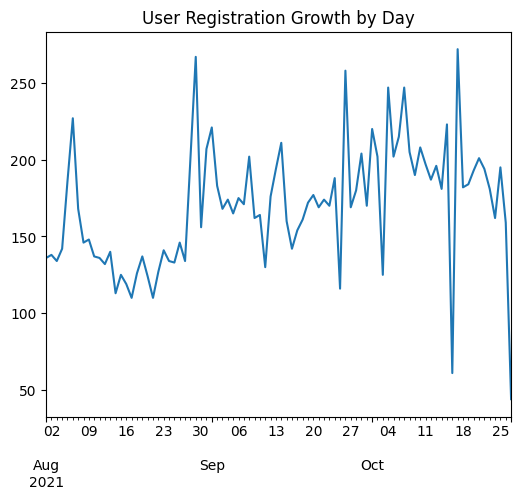
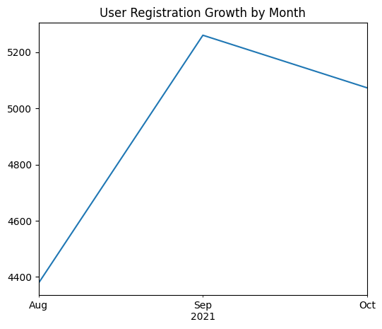
In the daily registration chart, we can see that October is the month with the
lowest and highest number of registrations,
meanwhile when we try to visualise it on monthly basis we can see that September is the month
with the highest number of registration, around 5200 users signed up.
Next, we want to see the comparison by user's gender.
gender = user[['user_id', 'user_gender']].groupby('user_gender').count()
		plt.pie(gender.user_id, labels=gender.index , startangle=90, shadow=True,explode=(0.1, 0.1), autopct='%1.2f%%')
		plt.title('Users\' Gender Distribution')
plt.show() 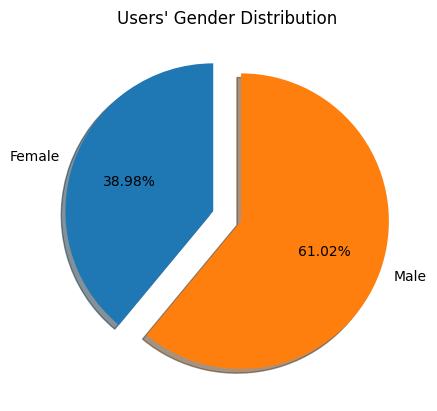
The user's gender distribution chart show that around 61.02% of our users are
male, meanwhile the rest are female.
Then we will try to visualise the user's range and source of income to see more details of it.
fig, ax = plt.subplots(figsize=(8, 8), subplot_kw=dict(aspect="equal"))
		income_source = user[['user_id', 'user_income_source']].groupby('user_income_source').count
		def func(pct, allvals):
			absolute = int(np.round(pct/100.*np.sum(allvals)))
			return "{:.1f}%\n({:d} users)".format(pct, absolute)

		wedges, texts, autotexts = ax.pie(income_source.user_id, autopct=lambda pct: func(pct, income_source.user_id),
			textprops=dict(color="black"), explode=(1,0,0,0,0,0,0,0,0,0))
		ax.legend(wedges, income_source.index,
			title="Income Source",
			loc="upper left",
			bbox_to_anchor=(1, 0, 0.5, 1))
		plt.setp(autotexts, size=8, weight="bold")
		ax.set_title("User's Income Source")
plt.show() 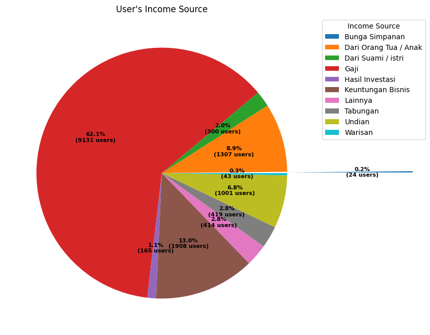
We read the chart counterclockwise starting from the exploded pie.
It shows that the lowest income source is from Bunga Simpanan (Saving's interest) with 0.2%.
whilst the majority of the income source is from Gaji (Salary) with 62.1% or equal to 9131
users.
Then we will see for the user's income range.
fig, ax = plt.subplots(figsize=(6, 5))
		ax = sns.countplot(y= user.user_income_range, data = user)

		ax.set_title('User Income Range')
		for x in ax.containers:
			ax.bar_label(x, label_type='edge')

plt.show() 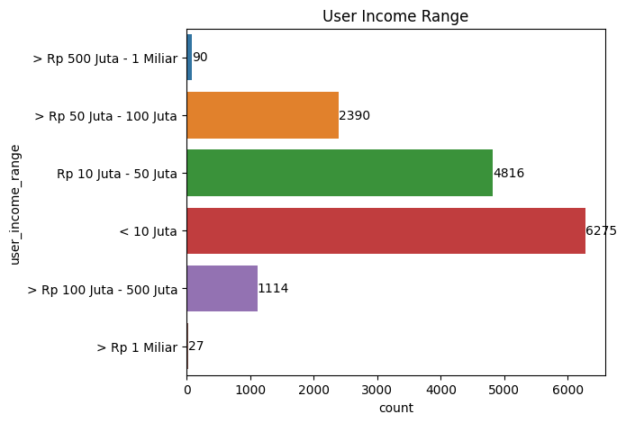
The user income range chart shows that the majority of users' income range is less than 10 Million Rupiah (approx 630 USD) with 6275 users.
Nevertheless, there are 27 users with the highest income range - 1 Billion Rupiah (approx 63000 USD) which is our potential big investor.
We also will try to combine income sources and range to see the breakdown of it.
fig, ax = plt.subplots(figsize=(12, 8))
		ax = sns.countplot(y= user.user_income_source, hue=user.user_income_range, data = user)
		ax.set_title('Income source and range')
		for x in ax.containers:
			ax.bar_label(x, label_type='edge')
		ax.legend(loc='best', fontsize=8)
		plt.show()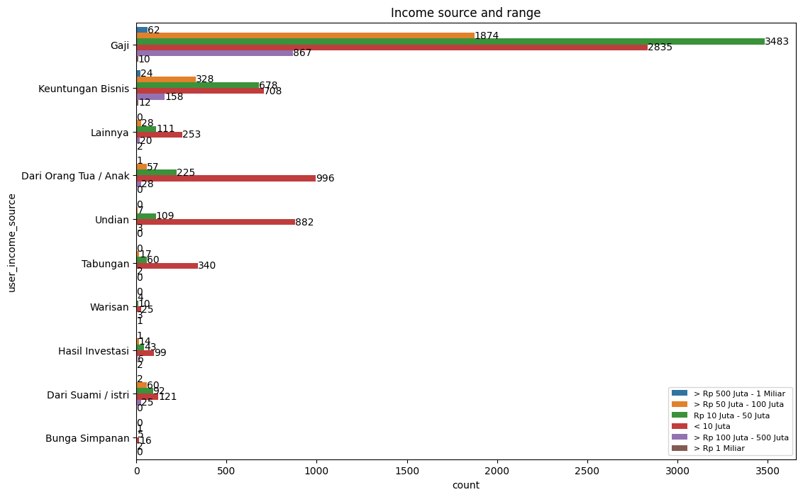
From the income range and source chart, we can see that 2835 of our users had wages of less than 10 Million Rupiah.
Moreover, the majority of our user's salary income range is between 10 Million to 50 Million Rupiah with a total of 3483 users.
It is noticeable that there are 10 users had a salary of more than 1 Billion Rupiah.
We will try to visualise the distribution of our user's occupations.
fig, ax = plt.subplots(figsize=(10, 5))
		ax =sns.countplot(x=user.user_occupation)
		for x in ax.containers:
			ax.bar_label(x, label_type='edge')
		ax.set_title('User occupation')
		plt.show()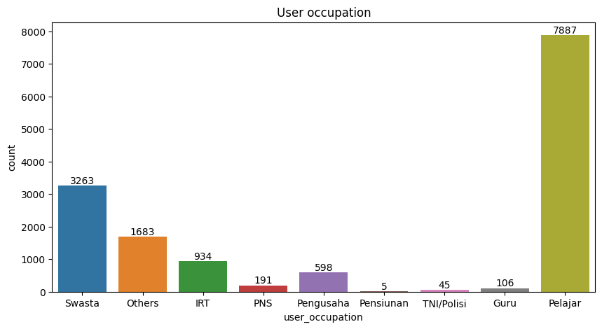
The users' occupation chart shows that the majority of our users are Pelajar
(Student) with a total of 7887 users.
Which is make sense that our majority income range is less than 10 Million.
We will try to combine the income range and user occupation to see more details about it.
fig, ax = plt.subplots(figsize=(12, 8))
		ax = sns.countplot(y= user.user_occupation, hue=user.user_income_range, data = user)
		ax.set_title('Income range and occupation')
		for x in ax.containers:
			ax.bar_label(x, label_type='edge')
		ax.legend(loc='right', fontsize=8)
		plt.show()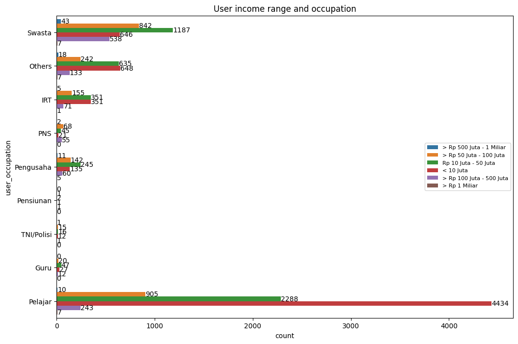
When we combined the income range and occupation, we found interesting
information that we have 17 students with an income range of more than 500 Million Rupiah.
So we will investigate a little bit further about the 17 students.
pelajar_age = user.query('user_occupation == \'Pelajar\' and (user_income_range == \'> Rp 500 Juta - 1 Miliar\'
sor user_income_range == \'> Rp 1 Miliar\')')| user_id | registration_import_datetime | user_gender | user_age | user_occupation | user_income_range | referral_code_used | user_income_source | registration_month | |
|---|---|---|---|---|---|---|---|---|---|
| 619 | 4228712 | 2021-10-05 | Male | 17 | Pelajar | > Rp 1 Miliar | used referral | Keuntungan Bisnis | 2021-10-31 |
| 899 | 3795261 | 2021-08-08 | Male | 18 | Pelajar | > Rp 1 Miliar | used referral | Lainnya | 2021-08-31 |
| 1394 | 4376258 | 2021-10-19 | Male | 18 | Pelajar | > Rp 500 Juta - 1 Miliar | used referral | Gaji | 2021-10-31 |
| 2282 | 3818578 | 2021-08-16 | Male | 19 | Pelajar | > Rp 1 Miliar | None | Keuntungan Bisnis | 2021-08-31 |
| 2609 | 3742646 | 2021-08-09 | Female | 20 | Pelajar | > Rp 1 Miliar | None | Keuntungan Bisnis | 2021-08-31 |
| 3999 | 3749935 | 2021-08-04 | Female | 21 | Pelajar | > Rp 1 Miliar | None | Keuntungan Bisnis | 2021-08-31 |
| 4076 | 4245492 | 2021-10-07 | Female | 21 | Pelajar | > Rp 500 Juta - 1 Miliar | None | Keuntungan Bisnis | 2021-10-31 |
| 4569 | 4355874 | 2021-10-17 | Male | 21 | Pelajar | > Rp 1 Miliar | used referral | Keuntungan Bisnis | 2021-10-31 |
| 6135 | 4239037 | 2021-10-06 | Female | 23 | Pelajar | > Rp 500 Juta - 1 Miliar | used referral | Gaji | 2021-10-31 |
| 8322 | 4371352 | 2021-10-19 | Male | 25 | Pelajar | > Rp 500 Juta - 1 Miliar | used referral | Gaji | 2021-10-31 |
| 8871 | 3959126 | 2021-09-02 | Female | 26 | Pelajar | > Rp 500 Juta - 1 Miliar | used referral | Keuntungan Bisnis | 2021-09-30 |
| 9063 | 4342801 | 2021-10-17 | Male | 26 | Pelajar | > Rp 500 Juta - 1 Miliar | None | Gaji | 2021-10-31 |
| 9725 | 4270298 | 2021-10-09 | Female | 27 | Pelajar | > Rp 500 Juta - 1 Miliar | None | Keuntungan Bisnis | 2021-10-31 |
| 10101 | 4134537 | 2021-09-24 | Male | 28 | Pelajar | > Rp 500 Juta - 1 Miliar | None | Keuntungan Bisnis | 2021-09-30 |
| 10925 | 4338825 | 2021-10-15 | Male | 29 | Pelajar | > Rp 1 Miliar | used referral | Lainnya | 2021-10-31 |
| 11617 | 4164878 | 2021-10-02 | Male | 31 | Pelajar | > Rp 500 Juta - 1 Miliar | used referral | Keuntungan Bisnis | 2021-10-31 |
| 11950 | 3858112 | 2021-08-18 | Female | 32 | Pelajar | > Rp 500 Juta - 1 Miliar | None | Gaji | 2021-08-31 |
It's interesting that we have a few users aged below 20, as a student with
an income range above 500 Million Rupiah and the income source is from business profit.
There is a possibility with the wrong information the user provided.
However, we just leave it as is for now and take notes just in case we might need some
adjustments prior to building the model.
The next thing we want to check is how many per cent of our users registered using referral codes.
This might also will help to decide what type of campaign approach to increase the registration
number.
referral_code = user[['user_id', 'referral_code_used']].groupby('referral_code_used').count()
		plt.pie(referral_code.user_id, labels=referral_code.index, startangle=90, shadow=True,explode=(0.1, 0.1), autopct='%1.2f%%')
		plt.title('Referral Code Comparison')
		plt.show()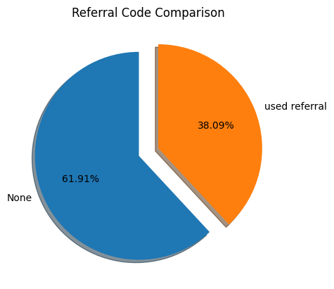
We can see from the referral code comparison that only 38.09% of our users use referral codes during their registration process.
We can create an announcement on the company website or application about bonus credit if the users refer some friends to register with us.
This will increase the number of new users, and transactions, and also a cheaper version of the advertisement as we announce it using our private platform so third-party advertisement costs are needed.
As well as encourage the current users to make more transactions using the bonus credit and so on.
We will check the average age of our users.
user['user_age'].describe()
			count    14712.000000
			mean        27.176591
			std          8.552585
			min         17.000000
			25%         21.000000
			50%         25.000000
			75%         31.000000
			max         83.000000
			Name: user_age, dtype: float64
The description shows that the average age of our users is 27 years old. The youngest is 17 and the oldest is 83 years old.
We will try to visualise its distribution of it by using the histogram.
user['user_age'].hist(figsize = (5,5))
		plt.title('User age distribution')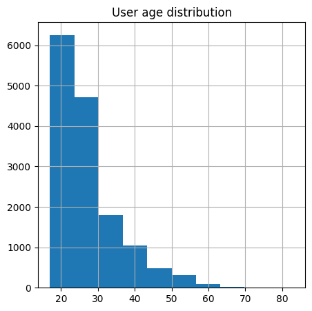
The histogram shows that most of our users are in the age group 20's and 30's.
The next step we will do is to use zscore to calculate if there are any outliers.
mean = np.mean(user.user_age)
		std = np.std(user.user_age)
		outlier = []
		for i in user.user_age:
			z = (i-mean)/std
			if z > 3:
				outlier.append(i)
		print('outliers in dataset are', set(outlier))
		sns.boxplot(x=user.user_age)
			outliers in dataset are {53, 54, 55, 56, 57, 58, 59, 60, 61, 62, 63, 64, 65, 66, 67, 69, 71, 73, 74, 76, 82, 83}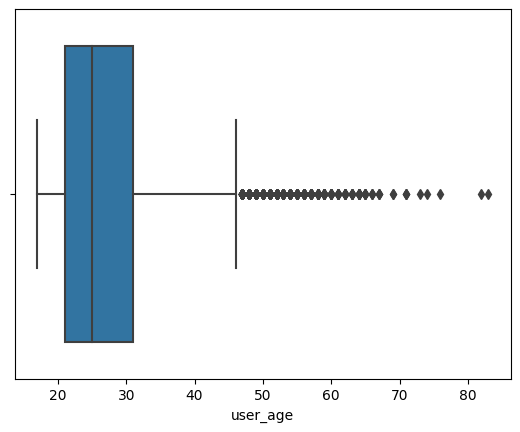
The z-score calculation, shows the outliers from the user's age are 53 years and older.
We will visualise the distribution and check how many users are in the outliers then merge dataset 1 and the transactions' dataset to see how many percentages of the outlier's users contribute to the transaction before we decide to remove the outliers or just leave it as is.
user_outliers = user.loc[user.user_age>=53,:]
		total_out = user_outliers.user_id.count()
		percentage_outliers = (total_out/total_user)
		print(f'Total users in outliers : {total_out} OR {percentage_outliers:.2%} from total user')
		fig, ax = plt.subplots(figsize=(6, 5))
		ax = sns.countplot(y= user_outliers.user_age, data = user_outliers)
		ax.set_title('User distribution above 53 years of age')
		for x in ax.containers:
			ax.bar_label(x, label_type='edge')
		plt.show()
			Total users in outliers : 264 OR 1.79% from total user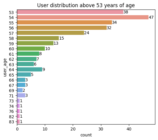
The chart above shows that we have a total of 264 users in the outliers category or equal to 1.79% of the total user.
With the highest distribution at 54 years of age and the lowest starting from 73 years. Since the age outliers are still in the normal scope, we will keep the users 54 years of age and older included in our analysis.
Transactions
We want to check how many rows of data we have on the transactions' dataset and the total number of users that making transactions.
print(f'Total rows: {trans.shape[0]} ,columns: {trans.shape[1]}')
transcation_users = trans['user_id'].nunique()
print(f'Total users making transaction period August - October 2021 = {transcation_users} users
	or {(transcation_users/total_user):.2%}')
trans.info()
	Total rows: 158811 ,columns: 14
	Total users making transaction period August - October 2021 = 8277 users or 56.26%
	RangeIndex: 158811 entries, 0 to 158810
	Data columns (total 14 columns):
	#   Column                               Non-Null Count   Dtype
	---  ------                               --------------   -----
	0   user_id                              158811 non-null  int64
	1   date                                 158811 non-null  object
	2   Saham_AUM                            106292 non-null  float64
	3   Saham_invested_amount                106292 non-null  float64
	4   Saham_transaction_amount             100839 non-null  float64
	5   Pasar_Uang_AUM                       131081 non-null  float64
	6   Pasar_Uang_invested_amount           131081 non-null  float64
	7   Pasar_Uang_transaction_amount        124273 non-null  float64
	8   Pendapatan_Tetap_AUM                 105946 non-null  float64
	9   Pendapatan_Tetap_invested_amount     105946 non-null  float64
	10  Pendapatan_Tetap_transaction_amount  100497 non-null  float64
	11  Campuran_AUM                         5352 non-null    float64
	12  Campuran_invested_amount             5352 non-null    float64
	13  Campuran_transaction_amount          5117 non-null    float64
	dtypes: float64(12), int64(1), object(1)
From the data description above, we can see that there are 158811 rows and 14 columns of data in the transactions' dataset.
Furthermore, it's only 8277 users made transactions or equal to 56.26% of the total users.
The company can create some campaigns to encourage new users to make new transactions.
In addition, we can see from the data information we have plenty of columns containing the null value.
We will check to confirm this information and change the 'date' column name to trans_date to avoid ambiguity with the method.
trans.rename(columns={"date": "trans_date"}, inplace=True)
trans['trans_date'] = pd.to_datetime(trans['trans_date'])
trans.isnull().sum()
	user_id                                     0
	trans_date                                  0
	Saham_AUM                               52519
	Saham_invested_amount                   52519
	Saham_transaction_amount                57972
	Pasar_Uang_AUM                          27730
	Pasar_Uang_invested_amount              27730
	Pasar_Uang_transaction_amount           34538
	Pendapatan_Tetap_AUM                    52865
	Pendapatan_Tetap_invested_amount        52865
	Pendapatan_Tetap_transaction_amount     58314
	Campuran_AUM                           153459
	Campuran_invested_amount               153459
	Campuran_transaction_amount            153694
	dtype: int64
The information above confirmed our findings and referring to the dataset information all of the columns with the null value is a transactions columns.
So, we will be changing the data to 0 instead of null.
trans.fillna(0, inplace=True)
trans.isnull().sum()
	user_id                                0
	trans_date                             0
	Saham_AUM                              0
	Saham_invested_amount                  0
	Saham_transaction_amount               0
	Pasar_Uang_AUM                         0
	Pasar_Uang_invested_amount             0
	Pasar_Uang_transaction_amount          0
	Pendapatan_Tetap_AUM                   0
	Pendapatan_Tetap_invested_amount       0
	Pendapatan_Tetap_transaction_amount    0
	Campuran_AUM                           0
	Campuran_invested_amount               0
	Campuran_transaction_amount            0
	dtype: int64
The null value has been replaced, in the next step, we will find how many times a transaction has been made by the user.
We will create some boolean flag column 1 if the user making a transaction on certain dates, and 0 if not. Later we will visualise this column to see the daily growth.
trans['count_saham'] = np.where(trans['Saham_transaction_amount']!=0.00,1,0)
trans['count_uang'] = np.where(trans['Pasar_Uang_transaction_amount']!=0.00,1,0)
trans['count_fixed'] = np.where(trans['Pendapatan_Tetap_transaction_amount']!=0.00,1,0)
trans['count_mixed'] = np.where(trans['Campuran_transaction_amount']!=0.00,1,0)

trans_count = trans[['count_saham', 'count_uang', 'count_fixed', 'count_mixed', 'trans_date']].groupby('trans_date').sum()
t_series = trans_count.index.to_pydatetime()

fig, ax = plt.subplots(figsize=(8, 6))

ax.plot(t_series, trans_count)
plt.title('Total transaction growth per day')
plt.legend(['Saham', 'Pasar Uang', 'Pendapatan Tetap', 'Campuran'])
plt.setp(ax.xaxis.get_ticklabels(), rotation=90)

plt.show()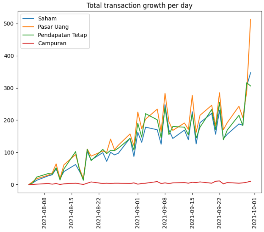
From the number of transactions chart, the higher type of transaction is Pasar Uang (Money Market) followed by Pendapatan Tetap (fixed income) and Saham (stocks) respectively.
As we can see from the dataset, the AUM and the invested amount is updated daily, meanwhile, transactions are filled when the users make any buy or sell transactions and it will fill with 0 if no transactions have been made.
Furthermore, we will be separating buy and sell transactions into new columns, to avoid biased data when summarising the transactions.
trans_buysell = ['Saham_transaction_amount','Pasar_Uang_transaction_amount', 'Pendapatan_Tetap_transaction_amount',
	'Campuran_transaction_amount']

for x in trans_buysell:
	mask = trans[x] < 0
	trans[x+'_buy'] = trans[x].mask(mask).abs()
	trans[x+'_sell'] = trans[x].mask(~mask).abs()

trans.loc[trans.Saham_transaction_amount !=0.00,:].head()| user_id | trans_date | Saham_AUM | Saham_invested_amount | Saham_transaction_amount | Pasar_Uang_AUM | Pasar_Uang_invested_amount | Pasar_Uang_transaction_amount | Pendapatan_Tetap_AUM | Pendapatan_Tetap_invested_amount | ... | count_fixed | count_mixed | Saham_transaction_amount_buy | Saham_transaction_amount_sell | Pasar_Uang_transaction_amount_buy | Pasar_Uang_transaction_amount_sell | Pendapatan_Tetap_transaction_amount_buy | Pendapatan_Tetap_transaction_amount_sell | Campuran_transaction_amount_buy | Campuran_transaction_amount_sell | |
|---|---|---|---|---|---|---|---|---|---|---|---|---|---|---|---|---|---|---|---|---|---|
| 25 | 50961 | 2021-09-01 | 1705566.0 | 1700000.0 | 1000000.0 | 100065.0 | 100000.0 | 0.0 | 200124.0 | 200000.0 | ... | 0 | 0 | 1000000.0 | NaN | 0.0 | NaN | 0.0 | NaN | 0.0 | NaN |
| 46 | 50961 | 2021-09-30 | 2063909.0 | 2000000.0 | 300000.0 | 700603.0 | 700000.0 | 600000.0 | 1398998.0 | 1400000.0 | ... | 1 | 0 | 300000.0 | NaN | 600000.0 | NaN | 1200000.0 | NaN | 0.0 | NaN |
| 102 | 61414 | 2021-08-13 | 0.0 | 0.0 | -10000.0 | 0.0 | 0.0 | 0.0 | 0.0 | 0.0 | ... | 0 | 0 | NaN | 10000.0 | 0.0 | NaN | 0.0 | NaN | 0.0 | NaN |
| 154 | 66145 | 2021-09-29 | 248015.0 | 240000.0 | 140000.0 | 29992.0 | 30000.0 | 0.0 | 129929.0 | 130000.0 | ... | 0 | 0 | 140000.0 | NaN | 0.0 | NaN | 0.0 | NaN | 0.0 | NaN |
| 166 | 67251 | 2021-09-20 | 562777.0 | 570000.0 | 530000.0 | 110065.0 | 110000.0 | 100000.0 | 420268.0 | 420000.0 | ... | 1 | 0 | 530000.0 | NaN | 100000.0 | NaN | 370000.0 | NaN | 0.0 | NaN |
5 rows × 26 columns
Since we split the transactions into buy and sell, we will drop the original
transaction column.
trans.drop(trans_buysell, axis=1, inplace=True)
trans.head()| user_id | trans_date | Saham_AUM | Saham_invested_amount | Pasar_Uang_AUM | Pasar_Uang_invested_amount | Pendapatan_Tetap_AUM | Pendapatan_Tetap_invested_amount | Campuran_AUM | Campuran_invested_amount | ... | count_fixed | count_mixed | Saham_transaction_amount_buy | Saham_transaction_amount_sell | Pasar_Uang_transaction_amount_buy | Pasar_Uang_transaction_amount_sell | Pendapatan_Tetap_transaction_amount_buy | Pendapatan_Tetap_transaction_amount_sell | Campuran_transaction_amount_buy | Campuran_transaction_amount_sell | |
|---|---|---|---|---|---|---|---|---|---|---|---|---|---|---|---|---|---|---|---|---|---|
| 0 | 50701 | 2021-08-30 | 0.0 | 0.0 | 0.0 | 0.0 | 0.0 | 0.0 | 10132277.0 | 10000000.0 | ... | 0 | 0 | 0.0 | NaN | 0.0 | NaN | 0.0 | NaN | 0.0 | NaN |
| 1 | 50701 | 2021-08-31 | 0.0 | 0.0 | 0.0 | 0.0 | 0.0 | 0.0 | 10206945.0 | 10000000.0 | ... | 0 | 0 | 0.0 | NaN | 0.0 | NaN | 0.0 | NaN | 0.0 | NaN |
| 2 | 50701 | 2021-09-01 | 0.0 | 0.0 | 0.0 | 0.0 | 0.0 | 0.0 | 9956556.0 | 10000000.0 | ... | 0 | 0 | 0.0 | NaN | 0.0 | NaN | 0.0 | NaN | 0.0 | NaN |
| 3 | 50701 | 2021-09-02 | 0.0 | 0.0 | 0.0 | 0.0 | 0.0 | 0.0 | 9914858.0 | 10000000.0 | ... | 0 | 0 | 0.0 | NaN | 0.0 | NaN | 0.0 | NaN | 0.0 | NaN |
| 4 | 50701 | 2021-09-03 | 0.0 | 0.0 | 0.0 | 0.0 | 0.0 | 0.0 | 10016360.0 | 10000000.0 | ... | 0 | 0 | 0.0 | NaN | 0.0 | NaN | 0.0 | NaN | 0.0 | NaN |
5 rows × 22 columns
The next thing is we will visualise the buy-sell transactions to see the total amount of transactions growth.
buysell = trans[['Saham_transaction_amount_buy', 'Saham_transaction_amount_sell', 'Pasar_Uang_transaction_amount_buy', 'Pasar_Uang_transaction_amount_sell',
	'Pendapatan_Tetap_transaction_amount_buy', 'Pendapatan_Tetap_transaction_amount_sell','Campuran_transaction_amount_buy', 'Campuran_transaction_amount_sell',
	'trans_date']].groupby('trans_date').sum()
t_series = buysell.index.to_pydatetime()

fig, ax = plt.subplots(figsize=(8, 6))

ax.plot(t_series, buysell)
plt.title('Summaries buying and selling growth per day')
ax.legend(['Saham_transaction_amount_buy', 'Saham_transaction_amount_sell', 'Pasar_Uang_transaction_amount_buy', 'Pasar_Uang_transaction_amount_sell',
'Pendapatan_Tetap_transaction_amount_buy', 'Pendapatan_Tetap_transaction_amount_sell','Campuran_transaction_amount_buy', 'Campuran_transaction_amount_sell'],
bbox_to_anchor=(1,1.05))
plt.setp(ax.xaxis.get_ticklabels(), rotation=90)
plt.ticklabel_format(style='plain', axis='y')

plt.show()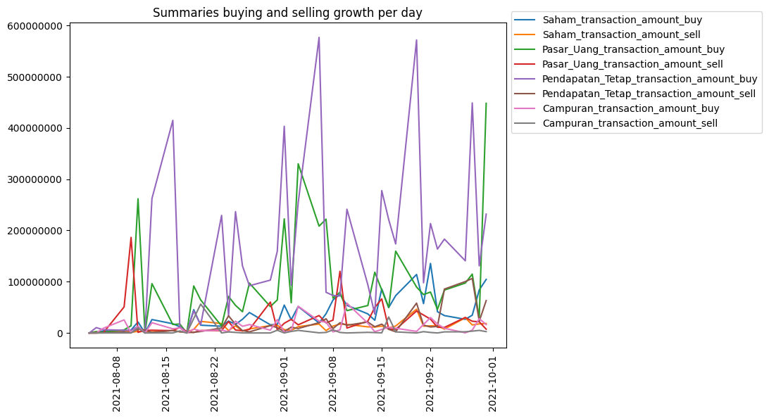
The summaries buying and selling chart shows that the total amount of Pendapatan Tetap (Buying) and Pasar Uang (Buying) are leading than other transactions.
We are also can see that the majority of the transactions are buying, this could meanings that our users are more interested in investing their money.
Since invested columns are updated daily with the last balanced of the users, we will drop the duplicate data and take the latest date.
Since invested columns are updated daily with the last balanced of the users, we will drop the duplicate data and take the latest date.
invested_col = ['user_id', 'trans_date', 'Saham_AUM', 'Saham_invested_amount', 'Pasar_Uang_AUM',
	'Pasar_Uang_invested_amount', 'Pendapatan_Tetap_AUM', 'Pendapatan_Tetap_invested_amount', 'Campuran_AUM',
	'Campuran_invested_amount']
invested_AUM = trans.sort_values(by='trans_date').drop_duplicates(subset=['user_id'], keep='last').reset_index(drop=True)
invested_AUM = invested_AUM[invested_col].copy()
print(f'Total rows: {invested_AUM.shape[0]}, columns: {invested_AUM.shape[1]}\nInvested:')
invested_AUM.head()
	Total rows: 8277, columns: 10
Invested:| user_id | trans_date | Saham_AUM | Saham_invested_amount | Pasar_Uang_AUM | Pasar_Uang_invested_amount | Pendapatan_Tetap_AUM | Pendapatan_Tetap_invested_amount | Campuran_AUM | Campuran_invested_amount | |
|---|---|---|---|---|---|---|---|---|---|---|
| 0 | 3786300 | 2021-09-30 | 0.00 | 0.00 | 0.00 | 0.00 | 0.00 | 0.00 | 0.00 | 0.00 |
| 1 | 3760891 | 2021-09-30 | 258975.00 | 249864.00 | 0.00 | 0.00 | 553302.00 | 550000.00 | 0.00 | 0.00 |
| 2 | 4096532 | 2021-09-30 | 13803192.00 | 13352136.00 | 2390277.00 | 2387932.00 | 8134491.00 | 8149154.00 | 0.00 | 0.00 |
| 3 | 2836295 | 2021-09-30 | 0.00 | 0.00 | 0.00 | 0.00 | 0.00 | 0.00 | 0.00 | 0.00 |
| 4 | 2839273 | 2021-09-30 | 0.00 | 0.00 | 10028.00 | 10000.00 | 0.00 | 0.00 | 0.00 | 0.00 |
Transactions dataframe:
sum_trans_total = trans.groupby('user_id')[['Saham_transaction_amount_buy',
	'Saham_transaction_amount_sell', 'Pasar_Uang_transaction_amount_buy',
	'Pasar_Uang_transaction_amount_sell',
	'Pendapatan_Tetap_transaction_amount_buy',
	'Pendapatan_Tetap_transaction_amount_sell',
	'Campuran_transaction_amount_buy', 'Campuran_transaction_amount_sell',
'count_saham', 'count_uang', 'count_fixed', 'count_mixed']].sum()
print(f'Total rows:{sum_trans_total.shape[0]}, columns: {sum_trans_total.shape[1]}\nTransactions:')
sum_trans_total.head()
	Total rows:8277, columns: 12
Transactions:| Saham_transaction_amount_buy | Saham_transaction_amount_sell | Pasar_Uang_transaction_amount_buy | Pasar_Uang_transaction_amount_sell | Pendapatan_Tetap_transaction_amount_buy | Pendapatan_Tetap_transaction_amount_sell | Campuran_transaction_amount_buy | Campuran_transaction_amount_sell | count_saham | count_uang | count_fixed | count_mixed | |
|---|---|---|---|---|---|---|---|---|---|---|---|---|
| user_id | ||||||||||||
| 50701 | 0.00 | 0.00 | 0.00 | 0.00 | 0.00 | 0.00 | 0.00 | 0.00 | 0 | 0 | 0 | 0 |
| 50961 | 1300000.00 | 0.00 | 600000.00 | 0.00 | 1200000.00 | 0.00 | 0.00 | 0.00 | 2 | 1 | 1 | 0 |
| 53759 | 0.00 | 0.00 | 0.00 | 0.00 | 0.00 | 0.00 | 0.00 | 0.00 | 0 | 0 | 0 | 0 |
| 54759 | 0.00 | 0.00 | 2000000.00 | 0.00 | 0.00 | 0.00 | 0.00 | 0.00 | 0 | 1 | 0 | 0 |
| 61414 | 0.00 | 10000.00 | 0.00 | 0.00 | 0.00 | 0.00 | 0.00 | 0.00 | 1 | 0 | 0 | 0 |
After creating the invested and transactions dataframe, then we will merge both
dataframe into new_trans and we will be using this dataset in the future.
new_trans = invested_AUM.merge(sum_trans_total, on='user_id')
print(f'Total rows: {new_trans.shape[0]}, columns:{new_trans.shape[1]}')
del invested_AUM, sum_trans_total
new_trans.head()
Total rows: 8277, columns:22| user_id | trans_date | Saham_AUM | Saham_invested_amount | Pasar_Uang_AUM | Pasar_Uang_invested_amount | Pendapatan_Tetap_AUM | Pendapatan_Tetap_invested_amount | Campuran_AUM | Campuran_invested_amount | ... | Pasar_Uang_transaction_amount_buy | Pasar_Uang_transaction_amount_sell | Pendapatan_Tetap_transaction_amount_buy | Pendapatan_Tetap_transaction_amount_sell | Campuran_transaction_amount_buy | Campuran_transaction_amount_sell | count_saham | count_uang | count_fixed | count_mixed | |
|---|---|---|---|---|---|---|---|---|---|---|---|---|---|---|---|---|---|---|---|---|---|
| 0 | 3786300 | 2021-09-30 | 0.00 | 0.00 | 0.00 | 0.00 | 0.00 | 0.00 | 0.00 | 0.00 | ... | 0.00 | 10000.00 | 0.00 | 0.00 | 0.00 | 0.00 | 1 | 1 | 0 | 0 |
| 1 | 3760891 | 2021-09-30 | 258975.00 | 249864.00 | 0.00 | 0.00 | 553302.00 | 550000.00 | 0.00 | 0.00 | ... | 310000.00 | 410000.00 | 499783.00 | 49783.00 | 0.00 | 0.00 | 5 | 7 | 7 | 0 |
| 2 | 4096532 | 2021-09-30 | 13803192.00 | 13352136.00 | 2390277.00 | 2387932.00 | 8134491.00 | 8149154.00 | 0.00 | 0.00 | ... | 1937932.00 | 0.00 | 6619154.00 | 0.00 | 0.00 | 0.00 | 2 | 1 | 2 | 0 |
| 3 | 2836295 | 2021-09-30 | 0.00 | 0.00 | 0.00 | 0.00 | 0.00 | 0.00 | 0.00 | 0.00 | ... | 0.00 | 100000.00 | 0.00 | 0.00 | 0.00 | 0.00 | 1 | 1 | 0 | 0 |
| 4 | 2839273 | 2021-09-30 | 0.00 | 0.00 | 10028.00 | 10000.00 | 0.00 | 0.00 | 0.00 | 0.00 | ... | 0.00 | 0.00 | 0.00 | 40000.00 | 0.00 | 0.00 | 1 | 0 | 1 | 0 |
The next thing we will do is to do a quick exploration of our bonds order dataset before combining it with user and transaction.
Bonds Order
print(f'Total rows: {result.shape[0]}, columns:{result.shape[1]}')
print(f'Total User: {result.user_id.nunique()}')
result.info()
	Total rows: 8484, columns:3
	Total User: 8484
	RangeIndex: 8484 entries, 0 to 8483
	Data columns (total 3 columns):
	#   Column              Non-Null Count  Dtype
	---  ------              --------------  -----
	0   user_id             8484 non-null   int64
	1   flag_order_bond     8484 non-null   int64
	2   bond_units_ordered  8484 non-null   int64
	dtypes: int64(3)
Since our problem statement is to find the prediction of whether the user will order bonds based on their behaviour.
We want to see the percentage that users who order bonds from the bonds order dataset to see the comparison between each class.
bond_order = result[['user_id', 'flag_order_bond']].groupby('flag_order_bond').count()
fig, ax = plt.subplots(figsize=(5, 5), subplot_kw=dict(aspect="equal"))
wedges, texts, autotexts = ax.pie(bond_order.user_id, autopct=lambda pct: func(pct, bond_order.user_id),
									textprops=dict(color="black"), explode=(0,0.1))
ax.legend(wedges, bond_order.index, title='Flag order bond', loc='upper right')
plt.show()

bond_chart=sns.countplot(x=result["flag_order_bond"])
plt.tight_layout()
plt.show()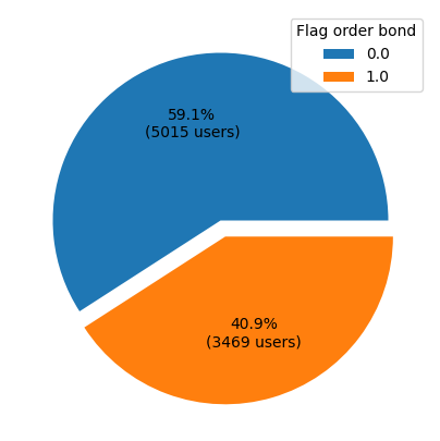
It shows that only 40.9% of our users order Government Bonds. However, we found a difference in our number of users from the transactions' dataset and 3. We have 8277 total users in the transactions dataset that makes transactions, meanwhile, 8484 users in the bonds order dataset.
We will combine the transactions' dataset and bonds in order to see the details of it.
trans_3 = result.merge(new_trans, how='left')
print(f'Total combined rows: {trans_3.shape[0]}, columns:{trans_3.shape[1]}')
print(f'Difference total users:{trans_3.user_id.nunique()-transaction_users}')
trans_3.isnull().sum()	Total combined rows: 8484, columns:24
	Difference total users:207

	user_id                                  0
	flag_order_bond                          0
	bond_units_ordered                       0
	trans_date                             207
	Saham_AUM                              207
	Saham_invested_amount                  207
	Pasar_Uang_AUM                         207
	Pasar_Uang_invested_amount             207
	Pendapatan_Tetap_AUM                   207
	Pendapatan_Tetap_invested_amount       207
	Campuran_AUM                           207
	Campuran_invested_amount               207
	Saham_transaction_amount               207
	Pasar_Uang_transaction_amount          207
	Pendapatan_Tetap_transaction_amount    207
	Campuran_transaction_amount            207
	dtype: int64
We left joined our dataset since our bonds order dataset has more rows of data for a better understanding what is the difference.
There are 8484 rows of data and 16 columns after the merging. We also check how much the difference between the dataset and the null value.
Our difference number of users between the transactions' dataset and 3 is 207 users, it is also the same as the number of our null values.
We will try to visualise the user with null values if they ordered bonds or not before we decide to exclude those users.
v = trans_3[trans_3.isnull().any(axis=1)]
v_null = v[['user_id', 'flag_order_bond']].groupby('flag_order_bond').count()
fig, ax = plt.subplots(figsize=(5, 5), subplot_kw=dict(aspect="equal"))
wedges, texts, autotexts = ax.pie(v_null.user_id, autopct=lambda pct: func(pct, v_null.user_id),
	textprops=dict(color="black"), explode=(0,1))
ax.legend(wedges, v_null.index, title='Null flag order bond', loc='upper right')
plt.show()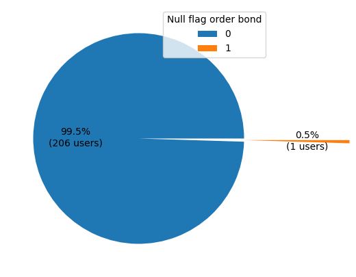
From the pie chart, we can see only 1 of 207 users ended up ordering bonds from the company.
Since we don't have any transactional records for the 207 users, it is safe to exclude them from our analysis.
Now, we will merge all of our datasets into 1 before we preprocess our data for modelling.
df1 = new_trans.merge(user, how='inner', on='user_id')
full_data = df1.merge(result, how='inner', on='user_id')
print(f'Total full rows: {full_data.shape[0]}, columns:{full_data.shape[1]}')
print('Null Values:')
full_data.isnull().sum()	Total full rows: 8277, columns:32

	Null Values:
	user_id                                     0
	trans_date                                  0
	Saham_AUM                                   0
	Saham_invested_amount                       0
	Pasar_Uang_AUM                              0
	Pasar_Uang_invested_amount                  0
	Pendapatan_Tetap_AUM                        0
	Pendapatan_Tetap_invested_amount            0
	Campuran_AUM                                0
	Campuran_invested_amount                    0
	Saham_transaction_amount_buy                0
	Saham_transaction_amount_sell               0
	Pasar_Uang_transaction_amount_buy           0
	Pasar_Uang_transaction_amount_sell          0
	Pendapatan_Tetap_transaction_amount_buy     0
	Pendapatan_Tetap_transaction_amount_sell    0
	Campuran_transaction_amount_buy             0
	Campuran_transaction_amount_sell            0
	count_saham                                 0
	count_uang                                  0
	count_fixed                                 0
	count_mixed                                 0
	registration_import_datetime                0
	user_gender                                 0
	user_age                                    0
	user_occupation                             0
	user_income_range                           0
	referral_code_used                          0
	user_income_source                          0
	registration_month                          0
	flag_order_bond                             0
	bond_units_ordered                          0
	dtype: int64
After we combined the 3 datasets, we have a total of 8277 rows of data and 32 columns.
We will create an age group bin into 17-19,20-29,30-39 and so on instead of user_age.
bins = [17, 20, 30, 40, 50, 60, 70, 80, 100]
labels = ['17-19','20-29','30-39', '40-49', '50-59', '60-69', '70-79', '80+']
full_data['age_group'] = pd.cut(full_data['user_age'], bins, labels = labels,include_lowest = True)
full_data.drop(['user_age'], axis=1, inplace=True)
full_data.age_group.unique()

	['20-29', '40-49', '30-39', '50-59', '17-19', '60-69', '70-79', '80+']
	Categories (8, object): ['17-19' < '20-29' < '30-39' < '40-49' < '50-59' < '60-69' < '70-79' < '80+']
trans_group = full_data[['age_group', 'Saham_transaction_amount_buy',
'Saham_transaction_amount_sell', 'Pasar_Uang_transaction_amount_buy',
'Pasar_Uang_transaction_amount_sell',
'Pendapatan_Tetap_transaction_amount_buy',
'Pendapatan_Tetap_transaction_amount_sell',
'Campuran_transaction_amount_buy', 'Campuran_transaction_amount_sell']].groupby('age_group').sum()
trans_group.plot(title='Summary transaction by age group', figsize=(8,5))
plt.ticklabel_format(axis='y', style='plain')
plt.show()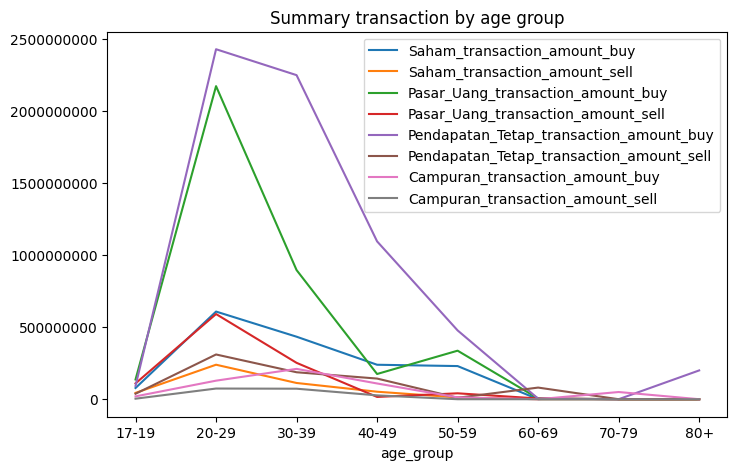
When we visualise the number of transactions mapped with the age group, we can see that the age group 20-29 years old contribute the most transactions, and it started to slow down until the user aged.
Then we will check the correlation from each of our features by plotting the correlation matrix.
Then we will check the correlation from each of our features by plotting the correlation matrix.
fig, ax = plt.subplots(figsize=(25,10))
sns.heatmap(full_data.corr(), annot = True, ax=ax, cmap = 'Blues')
plt.title("DataCorrelation")
plt.show()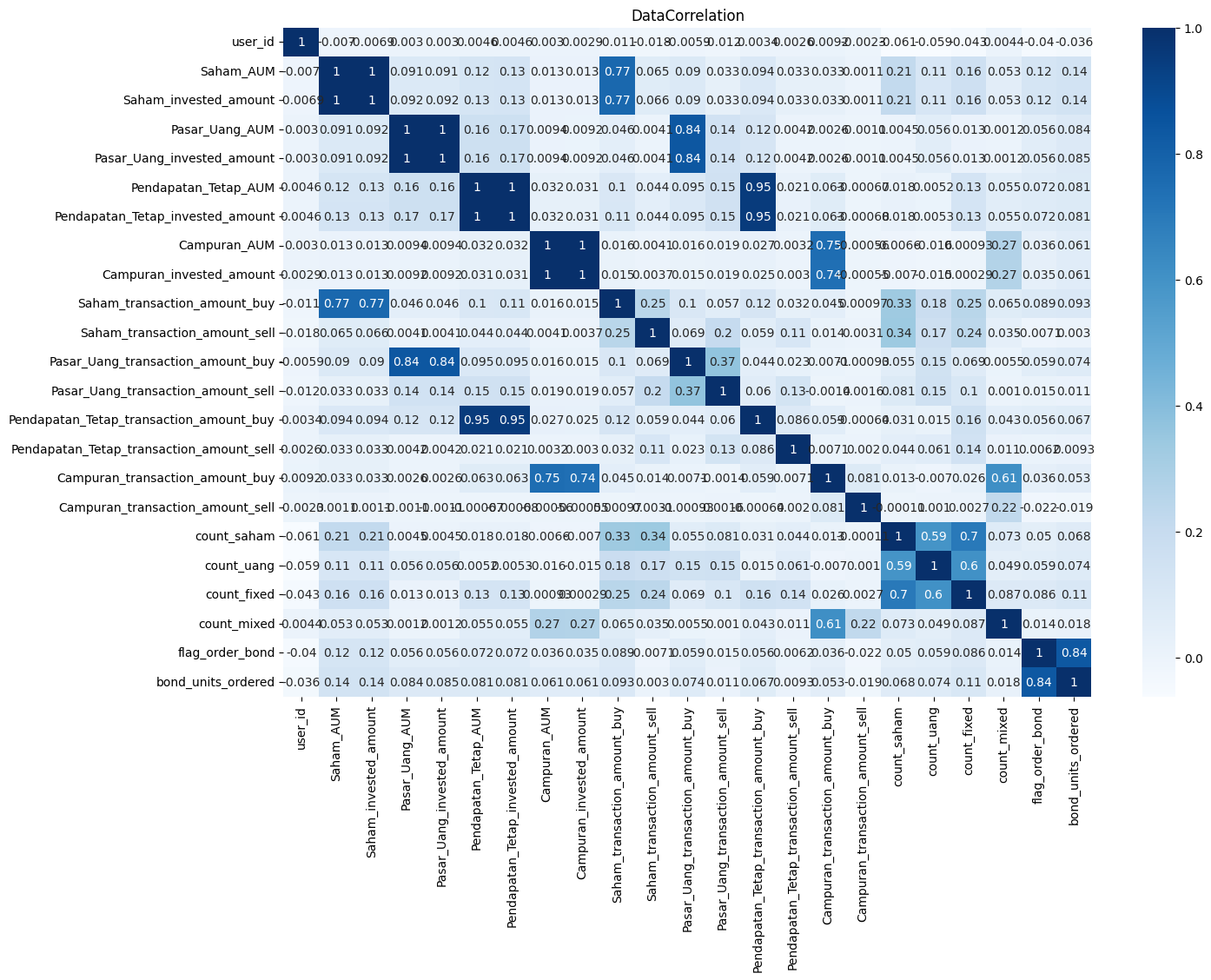
The correlation matrix shows that AUM and Invested column has a perfect positive correlation between each other as well as buying transactions.
Furthermore, bond_units_ordered also has a positive correlation with flag_order_bond. So, we will be dropping one of the features to avoid multicollinearity in the model performance.
pos_corr = ['Saham_AUM', 'Pasar_Uang_AUM', 'Pendapatan_Tetap_AUM', 'Campuran_AUM', 'Saham_transaction_amount_buy',
	'Pasar_Uang_transaction_amount_buy', 'Pendapatan_Tetap_transaction_amount_buy', 'Campuran_transaction_amount_buy',
	'bond_units_ordered']
full_data.drop(pos_corr, axis=1, inplace=True)
Preprocessing
So, we will convert our categorical data into numerical. We will print out the unique value from non-numerical data.
Moreover, we will remove the column transaction date, registration month, and user id.
for x in full_data:
	uniqueValues = full_data[x].unique()
	n_values = len(uniqueValues)
	if full_data[x].dtypes == object:
		print(f'Column: {x} -- total unique value: ({n_values}) {uniqueValues}')
	Column: user_gender -- total unique value: (2) ['Male' 'Female']
	Column: user_occupation -- total unique value: (9) ['Pelajar' 'Swasta' 'Others' 'Pengusaha' 'IRT' 'Guru' 'Pensiunan' 'PNS'
	'TNI/Polisi']
	Column: user_income_range -- total unique value: (6) ['< 10 Juta' 'Rp 10 Juta - 50 Juta' '> Rp 100 Juta - 500 Juta'
	'> Rp 500 Juta - 1 Miliar' '> Rp 50 Juta - 100 Juta' '> Rp 1 Miliar']
	Column: referral_code_used -- total unique value: (2) ['used referral' 'None']
	Column: user_income_source -- total unique value: (10) ['Keuntungan Bisnis' 'Gaji' 'Lainnya' 'Warisan' 'Undian'
	'Dari Orang Tua / Anak' 'Tabungan' 'Hasil Investasi' 'Dari Suami / istri'
	'Bunga Simpanan']
From the unique value details, it clearly shows that user_income_range is an ordinal category. So we will be using a label encoder to convert them into numerical data, meanwhile one hot encoding for the rest.
full_data.drop(['trans_date', 'registration_month', 'user_id'], axis=1, inplace=True)
one_hot_var = ['user_gender','user_occupation', 'referral_code_used', 'user_income_source']
one_hot = pd.get_dummies(full_data, columns = one_hot_var)

from sklearn.preprocessing import LabelEncoder

labelencoder = LabelEncoder()

one_hot['registration_import_datetime'] = labelencoder.fit_transform(one_hot['registration_import_datetime'])
one_hot['age_group'] = labelencoder.fit_transform(one_hot['age_group'])
one_hot['user_income_range'] = labelencoder.fit_transform(one_hot['user_income_range'])
one_hot.info()
	Int64Index: 8277 entries, 0 to 8276
	Data columns (total 39 columns):
	 #   Column                                    Non-Null Count  Dtype
	---  ------                                    --------------  -----
	 0   Saham_invested_amount                     8277 non-null   float64
	 1   Pasar_Uang_invested_amount                8277 non-null   float64
	 2   Pendapatan_Tetap_invested_amount          8277 non-null   float64
	 3   Campuran_invested_amount                  8277 non-null   float64
	 4   Saham_transaction_amount_sell             8277 non-null   float64
	 5   Pasar_Uang_transaction_amount_sell        8277 non-null   float64
	 6   Pendapatan_Tetap_transaction_amount_sell  8277 non-null   float64
	 7   Campuran_transaction_amount_sell          8277 non-null   float64
	 8   count_saham                               8277 non-null   int32
	 9   count_uang                                8277 non-null   int32
	 10  count_fixed                               8277 non-null   int32
	 11  count_mixed                               8277 non-null   int32
	 12  registration_import_datetime              8277 non-null   int32
	 13  user_income_range                         8277 non-null   int32
	 14  flag_order_bond                           8277 non-null   int64
	 15  age_group                                 8277 non-null   int32
	 16  user_gender_Female                        8277 non-null   uint8
	 17  user_gender_Male                          8277 non-null   uint8
	 18  user_occupation_Guru                      8277 non-null   uint8
	 19  user_occupation_IRT                       8277 non-null   uint8
	 20  user_occupation_Others                    8277 non-null   uint8
	 21  user_occupation_PNS                       8277 non-null   uint8
	 22  user_occupation_Pelajar                   8277 non-null   uint8
	 23  user_occupation_Pengusaha                 8277 non-null   uint8
	 24  user_occupation_Pensiunan                 8277 non-null   uint8
	 25  user_occupation_Swasta                    8277 non-null   uint8
	 26  user_occupation_TNI/Polisi                8277 non-null   uint8
	 27  referral_code_used_None                   8277 non-null   uint8
	 28  referral_code_used_used referral          8277 non-null   uint8
	 29  user_income_source_Bunga Simpanan         8277 non-null   uint8
	 30  user_income_source_Dari Orang Tua / Anak  8277 non-null   uint8
	 31  user_income_source_Dari Suami / istri     8277 non-null   uint8
	 32  user_income_source_Gaji                   8277 non-null   uint8
	 33  user_income_source_Hasil Investasi        8277 non-null   uint8
	 34  user_income_source_Keuntungan Bisnis      8277 non-null   uint8
	 35  user_income_source_Lainnya                8277 non-null   uint8
	 36  user_income_source_Tabungan               8277 non-null   uint8
	 37  user_income_source_Undian                 8277 non-null   uint8
	 38  user_income_source_Warisan                8277 non-null   uint8
After we convert our non-numerical data into numeric, we can see our dataset shape is changed to 8277 rows and 39 columns.
We will use the current feature to create our model using multiple classification algorithms and evaluate which one gives the best performance.
So, we will take out the target variable which is flag_order_bond from our dataset and divide them into training (60% of total data) and 40% for validation and testing.
Also, we will scale our data between 0 and 1 using minmaxscaler from scikit-learn.
x_v1 = one_hot.drop(['flag_order_bond'], axis=1)
y_v1 = one_hot['flag_order_bond'].copy()
Function to split data into train, val and test also scalingfrom sklearn.model_selection import train_test_split
from sklearn.preprocessing import MinMaxScaler

def split_scaled(x,y):
	xtrain, xtemp, ytrain, ytemp = train_test_split(x, y, train_size=0.6, random_state=3)
	xvalid, xtest, yvalid, ytest = train_test_split(xtemp, ytemp, test_size=0.5, random_state=3)
	scale = MinMaxScaler()

	xtrain_scaled = scale.fit_transform(xtrain)
	xvalid_scaled = scale.fit_transform(xvalid)
	xtest_scaled = scale.fit_transform(xtest)
	return xtrain_scaled, ytrain, xvalid_scaled, yvalid, xtest_scaled, ytest
Function to evaluate modelsfrom sklearn.metrics import ConfusionMatrixDisplay, accuracy_score
from sklearn.metrics import confusion_matrix, roc_auc_score, roc_curve, log_loss
score_comp = []
def eval(model, name, x1, y1, x2, y2, x3,y3):
	#accuracy score
	predtrain = model.predict(x1)
	predvalid = model.predict(x2)
	predtest = model.predict(x3)
	acctest = (accuracy_score(y3, predtest))
	accvalid = (accuracy_score(y2, predvalid))
	acctrain = (accuracy_score(y1, predtrain))
	overfit = acctrain - acctest

	tn, fp, fn, tp = confusion_matrix(y3, predtest).ravel()
	precision1 = (tp / (tp+fp))
	precision0 = (tn/(tn+fn))
	recall1 = (tp/(tp+fn))
	recall0 = (tn/(tn+fp))
	f1 = 2*(precision1 * recall1)/(precision1 + recall1)

	#log loss
	logtest = log_loss(y3,predtest)
	logtrain = log_loss(y1,predtrain)

	#roc auc score
	test_prob = model.predict_proba(x3)[::,1]
	train_prob = model.predict_proba(x1)[::,1]
	roctest = (roc_auc_score(y3, test_prob))
	roctrain = (roc_auc_score(y1, train_prob))
	fpr_test, tpr_test, _ = roc_curve(y3,  test_prob)
	fpr_train, tpr_train, _ = roc_curve(y1,  train_prob)

	#print report
	print(f'Training accuracy: {acctrain:.2%} \nValidation accuracy: {accvalid:.2%}\nTesting accuracy: {acctest:.2%} \nOverfitting: {overfit:.2%}')
	print(f'Log Loss Training: {logtrain}, Log Loss Testing: {logtest}')
	print(f'Precision class 1: {precision1:.2%} \nPrecision class 0: {precision0:.2%}')
	print(f'Recall class 1: {recall1:.2%} \nRecall class 0: {recall0:.2%}')
	print(f'F1: {f1:.2%}')
	print(f'ROC AUC Training: {roctrain:.2%} Testing: {roctest:.2%}')

	#insert result to list for comparison
	score_comp.append([name, acctrain, accvalid, acctest, overfit, precision1, precision0, recall1, recall0,
	f1, logtrain, logtest, roctrain, roctest])

	#confusion matrix plot
	disp = ConfusionMatrixDisplay(confusion_matrix(y3, predtest),display_labels=model.classes_)
	disp.plot()
	plt.show()

	#roc auc learning curve plot
	plt.title("Area Under Curve")
	plt.plot(fpr_test,tpr_test,label="AUC Test="+str(roctest))
	plt.plot(fpr_train,tpr_train,label="AUC Train="+str(roctrain))
	plt.ylabel('True Positive Rate')
	plt.xlabel('False Positive Rate')
	plt.legend(loc=4)
	plt.grid(True)
	plt.show()
Model 1 - Logistic Regression
The first model that we will implement is using Logistic Regression with our original
dataset.
xtrain, ytrain, xvalid, yvalid, xtest, ytest = split_scaled(x_v1, y_v1)

from sklearn.linear_model import LogisticRegression

logreg = LogisticRegression()
logreg.fit(xtrain, ytrain)
eval(logreg, 'logreg1', xtrain, ytrain, xvalid, yvalid, xtest, ytest)
	Training accuracy: 63.25%
	Validation accuracy: 61.51%
	Testing accuracy: 62.02%
	Overfitting: 1.23%
	Log Loss Training: 13.246006330072253, Log Loss Testing: 13.690493950334956
	Precision class 1: 52.56%
	Precision class 0: 66.20%
	Recall class 1: 40.76%
	Recall class 0: 75.92%
	F1: 45.92%
	ROC AUC Training: 66.75% Testing: 64.66%
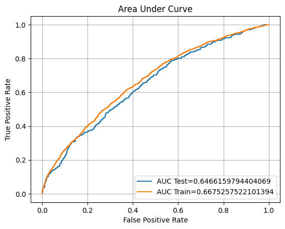
So, we can see that our model does not give a good accuracy score.
We will try to tune the model using GridSearch Cross Validation to improve the performance.
from sklearn.model_selection import GridSearchCV
log_param = [
	{
		'C': [0.01, 0.1, 1.0, 10, 100],
        'penalty': ['l1','l2'],
        'solver': ['newton-cg','saga'],
        'max_iter': [200,400,600,800]
	},
]

#tuned the model using gridsearch and kfold
opt_log = GridSearchCV(LogisticRegression(), param_grid = log_param, scoring='accuracy', cv=10, verbose = 2)
#fit the tuned model with training dataset
opt_log.fit(xtrain, ytrain)
print(opt_log.best_params_)
	{'C': 100, 'max_iter': 800, 'penalty': 'l1', 'solver': 'saga'}
We will fit our dataset to a new model with the parameters resulting from the Grid
Search.
lr = LogisticRegression(C= 100, penalty= 'l1', solver= 'saga', max_iter=800)
lr.fit(xtrain, ytrain)
eval(lr,'logreg_tuned', xtrain, ytrain, xvalid, yvalid, xtest, ytest)
	Training accuracy: 65.40%
	Validation accuracy: 63.63%
	Testing accuracy: 65.40%
	Overfitting: 0.01%
	Log Loss Training: 12.4693911644187, Log Loss Testing: 12.471626444422782
	Precision class 1: 58.01%
	Precision class 0: 68.71%
	Recall class 1: 45.34%
	Recall class 0: 78.52%
	F1: 50.90%
	ROC AUC Training: 70.22% Testing: 69.73%
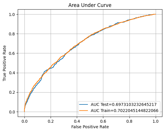
It seems the tuning increases the performance of the model. The next thing we will try to check the features coefficient and try to modify our features.
coefs_df = pd.DataFrame()
coefs_df['features'] = x_v1.columns
coefs_df['coefs'] = logreg.coef_[0]
print(coefs_df.sort_values('coefs', ascending=False).head(20))
plt.bar([x for x in range(len(coefs_df['coefs']))], coefs_df['coefs'])
plt.show()
						features  coefs
	0                      Saham_invested_amount   4.31
	1                 Pasar_Uang_invested_amount   2.63
	14                                 age_group   1.95
	10                               count_fixed   1.94
	2           Pendapatan_Tetap_invested_amount   1.58
	3                   Campuran_invested_amount   1.42
	30     user_income_source_Dari Suami / istri   0.59
	9                                 count_uang   0.57
	23                 user_occupation_Pensiunan   0.42
	36                 user_income_source_Undian   0.34
	12              registration_import_datetime   0.33
	20                       user_occupation_PNS   0.32
	26                   referral_code_used_None   0.26
	15                        user_gender_Female   0.23
	13                         user_income_range   0.20
	31                   user_income_source_Gaji   0.14
	29  user_income_source_Dari Orang Tua / Anak   0.12
	5         Pasar_Uang_transaction_amount_sell   0.09
	22                 user_occupation_Pengusaha   0.08
	25                user_occupation_TNI/Polisi   0.04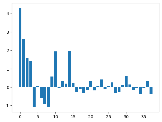
We will remove the low coefficient features that less than 0.2.
dropslv2 = coefs_df.loc[coefs_df['coefs']<0.2].features dropslv2 = dropslv2.to_list() encoded2 = one_hot.drop(dropslv2, axis=1) x_v2 = encoded2.drop(['flag_order_bond'], axis=1) y_v2 = encoded2['flag_order_bond'].copy()Fit new dataset to the modelxtrain2, ytrain2, xvalid2, yvalid2, xtest2, ytest2 = split_scaled(x_v2, y_v2) lr2 = LogisticRegression() lr2.fit(xtrain2, ytrain2) eval(lr2, 'logreg_coef', xtrain2, ytrain2, xvalid2, yvalid2, xtest2, ytest2)Training accuracy: 62.18% Validation accuracy: 61.27% Testing accuracy: 61.35% Overfitting: 0.83% Log Loss Training: 13.630684870068873, Log Loss Testing: 13.92991435328199 Precision class 1: 51.52% Precision class 0: 65.52% Recall class 1: 38.78% Recall class 0: 76.12% F1: 44.25% ROC AUC Training: 65.84% Testing: 64.27%
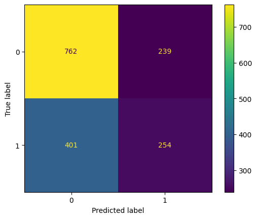
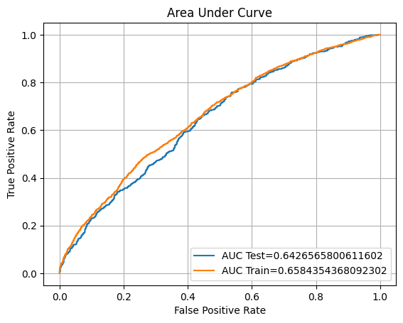
It seems that our previous model before removing the low coefficient features has a
better performance.
We will try to tune the model and see if the accuracy will improve.
from sklearn.model_selection import GridSearchCV
log_param = [
	{
		'C': [0.01, 0.1, 1.0, 10, 100],
		'penalty': ['l2', 'l1'],
		'solver': ['newton-cg', 'saga'],
		'max_iter': [200,400,600]
	},
]

#tuned the model using gridsearch and kfold
opt_log = GridSearchCV(LogisticRegression(), param_grid = log_param, scoring='accuracy', cv=10, verbose = 2)
#fit the tuned model with training dataset
opt_log.fit(xtrain2, ytrain2)
print(opt_log.best_params_) #best parameter tuning result
	{'C': 100, 'max_iter': 600, 'penalty': 'l1', 'solver': 'saga'}
Fit the model with new parameter from hypertuning.
lr3 = LogisticRegression(C=100, penalty='l1', solver='saga', max_iter=600)
lr3.fit(xtrain2, ytrain2)
eval(lr3, 'logreg_coef_tuned', xtrain2, ytrain2, xvalid2, yvalid2, xtest2, ytest2)
Training accuracy: 64.44%
Validation accuracy: 63.32%
Testing accuracy: 64.92%
Overfitting: -0.48%
Log Loss Training: 12.81777927611375, Log Loss Testing: 12.645750373838808
Precision class 1: 57.09%
Precision class 0: 68.52%
Recall class 1: 45.50%
Recall class 0: 77.62%
F1: 50.64%
ROC AUC Training: 69.33% Testing: 68.66%
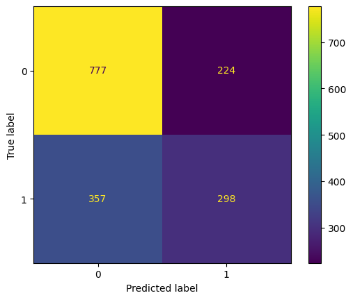
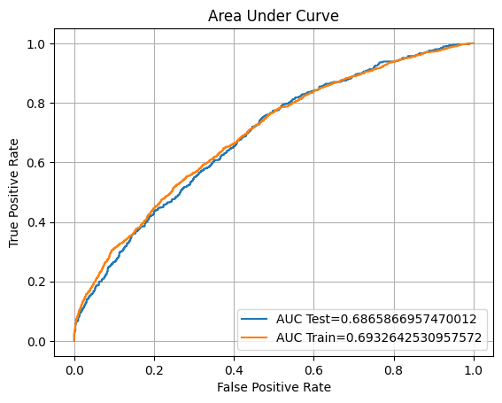
Unfortunately, when we reduce the low coefficient features it doesn't perform better
than our previous dataset.
We will try to create a new model using different algorithms.
Model 2 - Support Vector Machine
from sklearn.svm import SVC
svm_v1 = SVC(probability=True)
svm_v1.fit(xtrain, ytrain)
eval(svm_v1, 'svm1', xtrain, ytrain, xvalid, yvalid, xtest, ytest)
	Training accuracy: 63.85%
	Validation accuracy: 60.06%
	Testing accuracy: 61.11%
	Overfitting: 2.74%
	Log Loss Training: 13.028263760262844, Log Loss Testing: 14.016976317990002
	Precision class 1: 51.24%
	Precision class 0: 64.74%
	Recall class 1: 34.81%
	Recall class 0: 78.32%
	F1: 41.45%
	ROC AUC Training: 68.65% Testing: 62.84%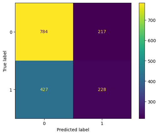
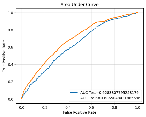
We will try to hyperparameter tuning our model to see if we can improve the
performance.
param_grid = [
		{
			'C': [0.01, 0.1, 1.0, 10, 100],
			'gamma': ['scale', 0.001, 0.01],
			'kernel': ['rbf','linear','sigmoid', 'poly']
		},
	]

	#tuned the model using gridsearch and kfold
	opt_log = GridSearchCV(SVC(), param_grid, scoring='accuracy', cv=10)
	#fit the tuned model with training dataset
	opt_log.fit(xtrain, ytrain)
	#best parameter tuning result
	print(opt_log.best_params_)
	{'C': 100, 'gamma': 'scale', 'kernel': 'poly'}
svm_v2 = SVC(probability=True, C=100, gamma='scale', kernel='poly')
svm_v2.fit(xtrain, ytrain)
eval(svm_v2, 'svm2', xtrain, ytrain, xvalid, yvalid, xtest, ytest)
Training accuracy: 70.18%
Validation accuracy: 61.93%
Testing accuracy: 63.83%
Overfitting: 6.35%
Log Loss Training: 10.749224862924386, Log Loss Testing: 13.037529215024863
Precision class 1: 55.45%
Precision class 0: 67.60%
Recall class 1: 43.51%
Recall class 0: 77.12%
F1: 48.76%
ROC AUC Training: 76.66% Testing: 65.07%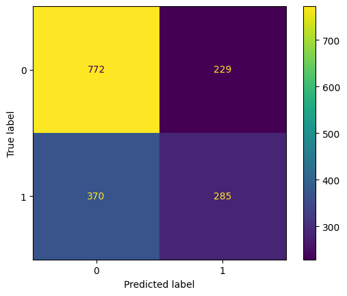
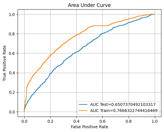
It seems that both of SVM model that we have created has an overfitting problem. After the
tuning, the accuracy score is increased but the overfitting is as well.
Model 3 - Random Forest Classifier
from sklearn.ensemble import RandomForestClassifier
			rf = RandomForestClassifier()
			rf.fit(xtrain, ytrain)
			eval(rf, 'random_forest', xtrain, ytrain, xvalid, yvalid, xtest, ytest)
				Training accuracy: 99.74%
				Validation accuracy: 67.49%
				Testing accuracy: 66.55%
				Overfitting: 33.19%
				Log Loss Training: 0.09435511358407653, Log Loss Testing: 12.058082112059724
				Precision class 1: 55.78%
				Precision class 0: 78.54%
				Recall class 1: 74.35%
				Recall class 0: 61.44%
				F1: 63.74%
				ROC AUC Training: 100.00% Testing: 76.33%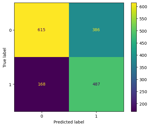
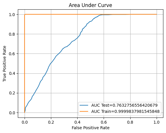
The Random Forest Classifier model results in an outstanding accuracy score with the training dataset.
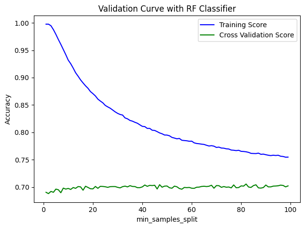
However, it does not have the same performance in the validation and testing dataset, which results in overfitting. Since it takes a lot of computation for the hyperparameter tuning, we will try to visualise the validation manually.
Function for calculate and visualise validation curve
			def validations(model, param, prange, x, y, k):
				train_scoreNum, test_scoreNum = validation_curve(
											model,
											X = x, y = y,
											param_name = param,
											param_range = prange, cv = k, scoring = "accuracy")
				# Calculating mean and standard deviation of training score
				mean_train_score = np.mean(train_scoreNum, axis = 1)
				std_train_score = np.std(train_scoreNum, axis = 1)

				# Calculating mean and standard deviation of testing score
				mean_test_score = np.mean(test_scoreNum, axis = 1)
				std_test_score = np.std(test_scoreNum, axis = 1)

				# Plot mean accuracy scores for training and testing scores
				plt.plot(prange, mean_train_score,
					label = "Training Score", color = 'b')
				plt.plot(prange, mean_test_score,
				label = "Cross Validation Score", color = 'g')

				# Creating the plot
				plt.title("Validation Curve with RF Classifier")
				plt.xlabel(param)
				plt.ylabel("Accuracy")
				plt.tight_layout()
				plt.legend(loc = 'best')
				plt.show()
			parameter_range = np.arange(1, 100, 1)
			validations(rf, 'min_samples_split', parameter_range, xtrain, ytrain, 10)
parameter_range = np.arange(1, 15, 1)
			validations(rf, 'max_depth', parameter_range, xtrain, ytrain, 10)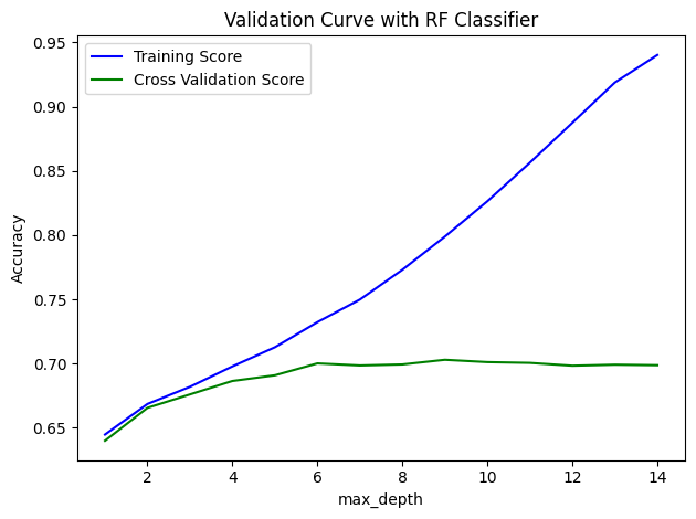
parameter_range = np.arange(1, 10, 1)
			validations(rf, 'n_estimators', parameter_range, xtrain, ytrain, 10)
validations(rf, 'min_samples_leaf', parameter_range, xtrain, ytrain, 10)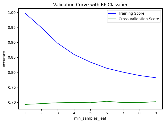
parameter_range = np.arange(1, 10, 1)
			validations(rf, 'max_features', parameter_range, xtrain, ytrain, 10)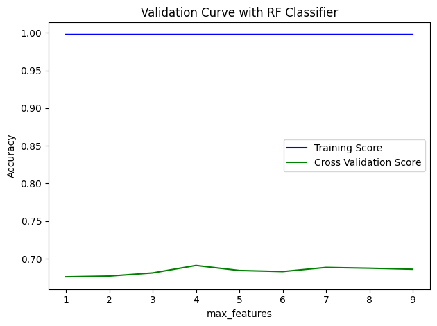
Fitting the parameter based on validation_curve visualisation
			RF_tuned = RandomForestClassifier(min_samples_split=100, max_depth=3, min_samples_leaf=15, n_estimators=1, max_features=7)
				RF_tuned.fit(xtrain, ytrain)
				eval(RF_tuned, 'rf_tuned', xtrain, ytrain, xvalid, yvalid, xtest, ytest)
				Training accuracy: 63.15%
				Validation accuracy: 62.48%
				Testing accuracy: 61.90%
				Overfitting: 1.25%
				Log Loss Training: 13.282296758373823, Log Loss Testing: 13.734024932688962
				Precision class 1: 51.35%
				Precision class 0: 74.09%
				Recall class 1: 69.62%
				Recall class 0: 56.84%
				F1: 59.11%
				ROC AUC Training: 68.15% Testing: 65.19%
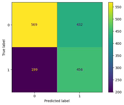
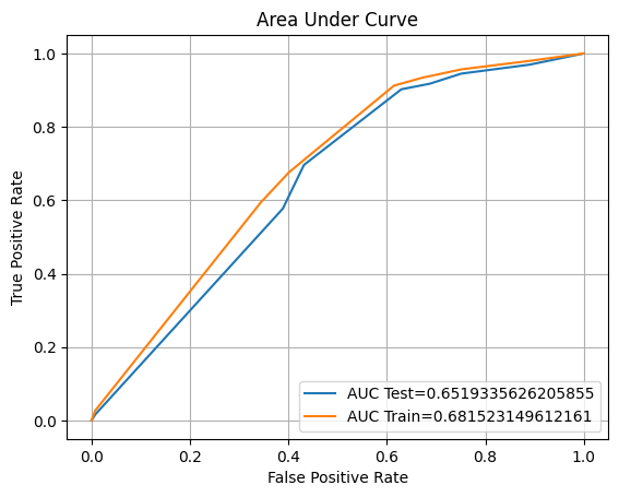
We successfully reduce the overfitting to 1.25% from our Random Forest algorithm from 33.19%. However, our accuracy score is also decreasing.
So, we will move on to our next model.
Model 4 - K-Nearest Neighbor Classifier
from sklearn.neighbors import KNeighborsClassifier
knn1 = KNeighborsClassifier()
knn1.fit(xtrain, ytrain)
eval(knn1, 'knn', xtrain, ytrain, xvalid, yvalid, xtest, ytest)
	Training accuracy: 72.51%
	Validation accuracy: 56.92%
	Testing accuracy: 58.82%
	Overfitting: 13.70%
	Log Loss Training: 9.907286926328014, Log Loss Testing: 14.84406498271612
	Precision class 1: 47.65%
	Precision class 0: 64.75%
	Recall class 1: 41.83%
	Recall class 0: 69.93%
	F1: 44.55%
	ROC AUC Training: 78.96% Testing: 58.57%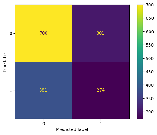
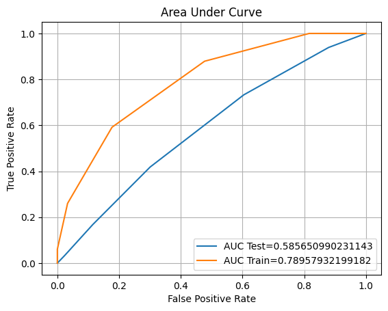
Our KNN model also has the same problem as our previous models. Furthermore, this model also yields the lowest accuracy score up to now.
We will do the same thing as our previous model with hyperparameter tuning.
#parameter dict
tuning_params = {
	'n_neighbors' : [19], #from the plot above
	"leaf_size":[5,10,20,30],
	"p":[1,2],
	'algorithm':['ball_tree', 'kd_tree', 'brute', 'auto']
}

#implement hyperparameter tuning to the model
opt_knn = GridSearchCV(KNeighborsClassifier(), param_grid = tuning_params, cv = 10, scoring='accuracy')
#fit the model with training dataset
opt_knn.fit(xtrain, ytrain)
print(opt_knn.best_params_){'algorithm': 'ball_tree', 'leaf_size': 10, 'n_neighbors': 19, 'p': 1}
knn_tuned = KNeighborsClassifier(leaf_size=10, n_neighbors=19, p=1, algorithm='ball_tree')
knn_tuned.fit(xtrain, ytrain)
eval(knn_tuned, 'knn_tuned', xtrain, ytrain, xvalid, yvalid, xtest, ytest)
Training accuracy: 65.18%
Validation accuracy: 58.91%
Testing accuracy: 59.66%
Overfitting: 5.52%
Log Loss Training: 12.54923010668215, Log Loss Testing: 14.539348106238078
Precision class 1: 48.77%
Precision class 0: 64.77%
Recall class 1: 39.39%
Recall class 0: 72.93%
F1: 43.58%
ROC AUC Training: 69.89% Testing: 61.47%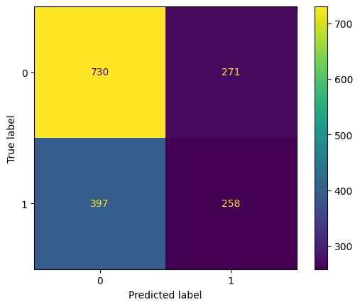
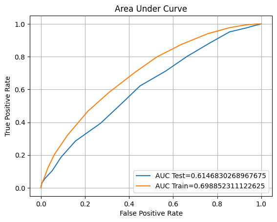
We were able to reduce the overfitting percentage and increase the accuracy score a little bit. It seems this model is the most underperformed compared to others.
Model 5 - Decision Tree Classifier
from sklearn.tree import DecisionTreeClassifier
dt = DecisionTreeClassifier()
dt.fit(xtrain, ytrain)
eval(dt, 'decision_tree', xtrain, ytrain, xvalid, yvalid, xtest, ytest)
	Training accuracy: 99.74%
	Validation accuracy: 65.26%
	Testing accuracy: 66.00%
	Overfitting: 33.74%
	Log Loss Training: 0.09435511358407653, Log Loss Testing: 12.253971532652752
	Precision class 1: 56.18%
	Precision class 0: 74.01%
	Recall class 1: 63.82%
	Recall class 0: 67.43%
	F1: 59.76%
	ROC AUC Training: 100.00% Testing: 65.68%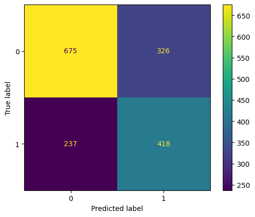
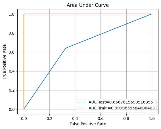
From the result above, it looks like decision tree has the similar results with random
forest Classifier.
random_tree = {'criterion': ['gini', 'entropy'],
	'max_depth': [int(x) for x in np.linspace(start = 1, stop = 20, num = 1)],
	'min_samples_split': [int(x) for x in np.linspace(start = 1, stop = 20, num = 1)],
	'min_samples_leaf': [int(x) for x in np.linspace(start = 1, stop = 20, num = 1)]}

#implement hyperparameter tuning to the model
opt_decTree = GridSearchCV(DecisionTreeClassifier(), param_grid= random_tree, cv = 10, scoring='accuracy')
#fit the model with training dataset
opt_decTree.fit(xtrain, ytrain)
print(opt_decTree.best_params_)
	{'criterion': 'gini', 'max_depth': 1, 'min_samples_leaf': 1, 'min_samples_split': 1}
dt_tuned = DecisionTreeClassifier(criterion='gini', max_depth=1, min_samples_leaf=1, min_samples_split=1)
dt_tuned.fit(xtrain, ytrain)
eval(dt_tuned, 'dt_tuned', xtrain, ytrain, xvalid, yvalid, xtest, ytest)
Training accuracy: 67.52%
Validation accuracy: 66.47%
Testing accuracy: 66.79%
Overfitting: 0.73%
Log Loss Training: 11.707292170085777, Log Loss Testing: 11.97102014735171
Precision class 1: 55.45%
Precision class 0: 82.54%
Recall class 1: 81.53%
Recall class 0: 57.14%
F1: 66.01%
ROC AUC Training: 69.48% Testing: 69.33%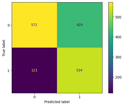
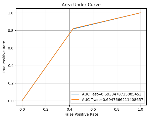
The hyperparameter tuning successfully lowers the overfitting percentage by more than 30% and slightly increases the accuracy score. We will implement our last algorithm before we compare which algorithm is performing better.
Model 6 - Naive Bayes
from sklearn.naive_bayes import GaussianNB
nb = GaussianNB()
nb.fit(xtrain, ytrain)
eval(nb, 'naive', xtrain, ytrain, xvalid, yvalid, xtest, ytest)
	Training accuracy: 62.00%
	Validation accuracy: 60.06%
	Testing accuracy: 63.10%
	Overfitting: -1.10%
	Log Loss Training: 13.696007641011693, Log Loss Testing: 13.298715109148901
	Precision class 1: 57.86%
	Precision class 0: 64.17%
	Recall class 1: 24.73%
	Recall class 0: 88.21%
	F1: 34.65%
	ROC AUC Training: 65.56% Testing: 64.16%

Unlike our other model, this model has an underfitting problem. We will perform the same procedure with hyperparameter tuning.
params_NB = {'var_smoothing': np.logspace(0,-9, num=100)}
opt = GridSearchCV(GaussianNB(), param_grid=params_NB, cv=10,verbose=1,scoring='accuracy')
opt.fit(xtrain, ytrain)
print(opt.best_params_)
	{'var_smoothing': 1.873817422860383e-08}
nbtuned = GaussianNB(var_smoothing=1.873817422860383e-08)
nbtuned.fit(xtrain, ytrain)
eval(nbtuned, 'naive_tuned', xtrain, ytrain, xvalid, yvalid, xtest, ytest)
Training accuracy: 62.08%
Validation accuracy: 60.12%
Testing accuracy: 62.92%
Overfitting: -0.84%
Log Loss Training: 13.666975298370438, Log Loss Testing: 13.36401158267991
Precision class 1: 57.19%
Precision class 0: 64.11%
Recall class 1: 24.89%
Recall class 0: 87.81%
F1: 34.68%
ROC AUC Training: 65.55% Testing: 64.13%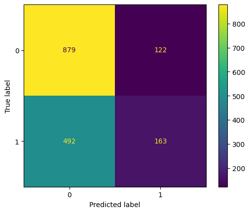
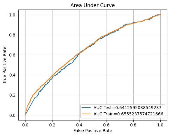
Unfortunately, our hyperparameter tuning does not give the best results. So we will compare all of our models and see which one performs better than the others.
Conclusion - Model Selection
We have been implementing 6 classification algorithms to our dataset for the bonds order prediction.
We will see which one has a better performance.
scores = pd.DataFrame(score_comp, columns=['Algorithm','accuracy_train','accuracy_valid','accuracy_test', 'overfit', 'precision1', 'precision0', 'recall1', 'recall0','f1','loss_train', 'loss_test', 'roc_train', 'roc_test'])
scores| Algorithm | accuracy_train | accuracy_valid | accuracy_test | overfit | precision1 | precision0 | recall1 | recall0 | f1 | loss_train | loss_test | roc_train | roc_test |
|---|---|---|---|---|---|---|---|---|---|---|---|---|---|
| logreg1 | 0.63 | 0.62 | 0.62 | 0.01 | 0.53 | 0.66 | 0.41 | 0.76 | 0.46 | 13.25 | 13.69 | 0.67 | 0.65 |
| logreg_tuned | 0.65 | 0.64 | 0.65 | 0.00 | 0.58 | 0.69 | 0.45 | 0.79 | 0.51 | 12.47 | 12.47 | 0.70 | 0.70 |
| logreg_coef | 0.62 | 0.61 | 0.61 | 0.01 | 0.52 | 0.66 | 0.39 | 0.76 | 0.44 | 13.63 | 13.93 | 0.66 | 0.64 |
| logreg_coef_tuned | 0.64 | 0.63 | 0.65 | -0.00 | 0.57 | 0.68 | 0.45 | 0.78 | 0.50 | 12.83 | 12.71 | 0.69 | 0.68 |
| svm1 | 0.64 | 0.60 | 0.61 | 0.03 | 0.51 | 0.65 | 0.35 | 0.78 | 0.41 | 13.03 | 14.02 | 0.69 | 0.63 |
| svm2 | 0.70 | 0.62 | 0.64 | 0.06 | 0.55 | 0.68 | 0.44 | 0.77 | 0.49 | 10.75 | 13.04 | 0.77 | 0.65 |
| random_forest | 1.00 | 0.67 | 0.67 | 0.33 | 0.56 | 0.79 | 0.74 | 0.61 | 0.64 | 0.09 | 12.06 | 1.00 | 0.76 |
| rf_tuned | 0.63 | 0.62 | 0.62 | 0.01 | 0.51 | 0.74 | 0.70 | 0.57 | 0.59 | 13.28 | 13.73 | 0.68 | 0.65 |
| knn | 0.73 | 0.57 | 0.59 | 0.14 | 0.48 | 0.65 | 0.42 | 0.70 | 0.45 | 9.91 | 14.84 | 0.79 | 0.59 |
| knn_tuned | 0.65 | 0.59 | 0.60 | 0.06 | 0.49 | 0.65 | 0.39 | 0.73 | 0.44 | 12.55 | 14.54 | 0.70 | 0.61 |
| decision_tree | 1.00 | 0.65 | 0.66 | 0.34 | 0.56 | 0.74 | 0.64 | 0.67 | 0.60 | 0.09 | 12.25 | 1.00 | 0.66 |
| dt_tuned | 0.68 | 0.66 | 0.67 | 0.01 | 0.55 | 0.83 | 0.82 | 0.57 | 0.66 | 11.71 | 11.97 | 0.69 | 0.69 |
| naive | 0.62 | 0.60 | 0.63 | -0.01 | 0.58 | 0.64 | 0.25 | 0.88 | 0.35 | 13.70 | 13.30 | 0.66 | 0.64 |
| naive_tuned | 0.62 | 0.60 | 0.63 | -0.01 | 0.57 | 0.64 | 0.25 | 0.88 | 0.35 | 13.67 | 13.36 | 0.66 | 0.64 |
From the score table above, we can see that KNN is the most less perform compare to others.
When we see how precise the model is in predicting class 1 and 0, it seems that logistic regression has a better performance compared to others.
However, the percentage of the score is not satisfying. If we can get more data to train our model, we could increase our accuracy score as the model has more data to learn.
For now, tuned logistic regression is our better option with a 65% accuracy score, 58% precision in class 1 and 69% precision in class 0.