Devy Ratnasari
Credit Card Fraud Detection
This is a group project from Durham College Capstone 1. Team members: Devy Ratnasari, Priyanka Singh, Gopika Shaji, Oluwole Ayodele, and Saurav Bisht. We used 5 different machine learning and 2 deep learning algorithms to classify transactions into fraud vs non-fraud. The datasets are dummy data from Kaggle and it has been split into 2 files, Train and Test. We combined 2 datasets to see the total number of data and the balance percentage before splitting it into train and test datasets.
EDA & Data Preprocessing
Exploratory Data Analysis is one of the major step to fine-tune the given dataset and performing data analysis to understand the insights of the key characteristics of various entities of the data set like column(s), row(s) by applying Pandas, NumPy, Statistical Methods, and Data visualization packages. Outcome of this phase are:
- Understanding and cleaning the given dataset.
- Understanding relationship between different features or columns and target variable.
- Provide guidelines for essential variables vs non-essential variables.
- Handling Missing values or human error.
- Identifying outliers.
#import the train dataset
dtrain = pd.read_csv('../dataset/fraudTrain.csv')

#import the test dataset
dtest = pd.read_csv('../dataset/fraudTest.csv')

#combine 2 datasets into 1
fullset = pd.concat([dtrain, dtest])

#delete the original data before merge to save memory
del dtrain, dtest

#see the structure of data
print(fullset.shape)
print(fullset.info())

#print sample of data(the first 5 rows)
fullset.head()
	(1852394, 23)
	Int64../index: 1852394 entries, 0 to 555718
	Data columns (total 23 columns):
	#   Column                 Dtype
	---  ------                 -----
	0   Unnamed: 0             int64
	1   trans_date_trans_time  object
	2   cc_num                 int64
	3   merchant               object
	4   category               object
	5   amt                    float64
	6   first                  object
	7   last                   object
	8   gender                 object
	9   street                 object
	10  city                   object
	11  state                  object
	12  zip                    int64
	13  lat                    float64
	14  long                   float64
	15  city_pop               int64
	16  job                    object
	17  dob                    object
	18  trans_num              object
	19  unix_time              int64
	20  merch_lat              float64
	21  merch_long             float64
	22  is_fraud               int64
dtypes: float64(5), int64(6), object(12)| Unnamed: 0 | trans_date_trans_time | cc_num | merchant | category | amt | first | last | gender | street | ... | lat | long | city_pop | job | dob | trans_num | unix_time | merch_lat | merch_long | is_fraud | |
|---|---|---|---|---|---|---|---|---|---|---|---|---|---|---|---|---|---|---|---|---|---|
| 0 | 0 | 2019-01-01 00:00:18 | 2703186189652095 | fraud_Rippin, Kub and Mann | misc_net | 4.97 | Jennifer | Banks | F | 561 Perry Cove | ... | 36.0788 | -81.1781 | 3495 | Psychologist, counselling | 1988-03-09 | 0b242abb623afc578575680df30655b9 | 1325376018 | 36.011293 | -82.048315 | 0 |
| 1 | 1 | 2019-01-01 00:00:44 | 630423337322 | fraud_Heller, Gutmann and Zieme | grocery_pos | 107.23 | Stephanie | Gill | F | 43039 Riley Greens Suite 393 | ... | 48.8878 | -118.2105 | 149 | Special educational needs teacher | 1978-06-21 | 1f76529f8574734946361c461b024d99 | 1325376044 | 49.159047 | -118.186462 | 0 |
| 2 | 2 | 2019-01-01 00:00:51 | 38859492057661 | fraud_Lind-Buckridge | entertainment | 220.11 | Edward | Sanchez | M | 594 White Dale Suite 530 | ... | 42.1808 | -112.2620 | 4154 | Nature conservation officer | 1962-01-19 | a1a22d70485983eac12b5b88dad1cf95 | 1325376051 | 43.150704 | -112.154481 | 0 |
| 3 | 3 | 2019-01-01 00:01:16 | 3534093764340240 | fraud_Kutch, Hermiston and Farrell | gas_transport | 45.00 | Jeremy | White | M | 9443 Cynthia Court Apt. 038 | ... | 46.2306 | -112.1138 | 1939 | Patent attorney | 1967-01-12 | 6b849c168bdad6f867558c3793159a81 | 1325376076 | 47.034331 | -112.561071 | 0 |
| 4 | 4 | 2019-01-01 00:03:06 | 375534208663984 | fraud_Keeling-Crist | misc_pos | 41.96 | Tyler | Garcia | M | 408 Bradley Rest | ... | 38.4207 | -79.4629 | 99 | Dance movement psychotherapist | 1986-03-28 | a41d7549acf90789359a9aa5346dcb46 | 1325376186 | 38.674999 | -78.632459 | 0 |
#convert dob to age
fullset['dob'] = pd.to_datetime(fullset.dob)
def from_dob_to_age(born):
	today = datetime.date.today()
	return today.year - born.year - ((today.month, today.day) < (born.month, born.day))

fullset['Age']=fullset['dob'].apply(lambda x: from_dob_to_age(x))
fig= plt.figure(figsize=(10,5) )
fig.add_subplot(1,3,1)
ar_6=sns.boxplot(x=fullset["is_fraud"],y=fullset["Age"])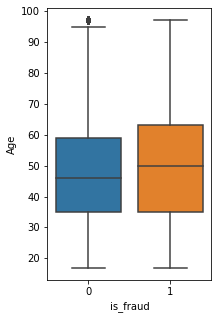
fullset.isna().sum()
	Unnamed: 0               0
	trans_date_trans_time    0
	cc_num                   0
	merchant                 0
	category                 0
	amt                      0
	first                    0
	last                     0
	gender                   0
	street                   0
	city                     0
	state                    0
	zip                      0
	lat                      0
	long                     0
	city_pop                 0
	job                      0
	dob                      0
	trans_num                0
	unix_time                0
	merch_lat                0
	merch_long               0
	is_fraud                 0
Age 0for col in fullset:
uValue = np.unique(fullset[col])
rValue = len(uValue)
if rValue < 50:
print('Unique values {} total {} --{}'.format(col, rValue, uValue))
else:
print('Unique Value {} -- {}'.format(col, rValue))
Unique Value Unnamed: 0 -- 1296675
Unique values trans_date_trans_time total 24 --[Period('2019-01', 'M') Period('2019-02', 'M') Period('2019-03', 'M')
Period('2019-04', 'M') Period('2019-05', 'M') Period('2019-06', 'M')
Period('2019-07', 'M') Period('2019-08', 'M') Period('2019-09', 'M')
Period('2019-10', 'M') Period('2019-11', 'M') Period('2019-12', 'M')
Period('2020-01', 'M') Period('2020-02', 'M') Period('2020-03', 'M')
Period('2020-04', 'M') Period('2020-05', 'M') Period('2020-06', 'M')
Period('2020-07', 'M') Period('2020-08', 'M') Period('2020-09', 'M')
Period('2020-10', 'M') Period('2020-11', 'M') Period('2020-12', 'M')]
Unique Value cc_num -- 999
Unique Value merchant -- 693
Unique values category total 14 --['entertainment' 'food_dining' 'gas_transport' 'grocery_net' 'grocery_pos'
'health_fitness' 'home' 'kids_pets' 'misc_net' 'misc_pos' 'personal_care'
'shopping_net' 'shopping_pos' 'travel']
Unique Value amt -- 60616
Unique Value first -- 355
Unique Value last -- 486
Unique values gender total 2 --['F' 'M']
Unique Value street -- 999
Unique Value city -- 906
Unique Value state -- 51
Unique Value zip -- 985
Unique Value lat -- 983
Unique Value long -- 983
Unique Value city_pop -- 891
Unique Value job -- 497
Unique Value dob -- 984
Unique Value trans_num -- 1852394
Unique Value unix_time -- 1819583
Unique Value merch_lat -- 1754157
Unique Value merch_long -- 1809753
Unique values is_fraud total 2 --[0 1]
Unique Value Age -- 80fraud = fullset.query('is_fraud == 1')
fraud['trans_date_trans_time'].value_counts().sort_../index().plot()
plt.title('Fraud growths')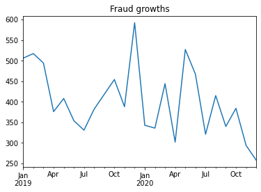
sns.countplot(y=fraud.category, data=fraud, palette = 'Set3')
plt.title('Fraud Category')
plt.xlabel('Total')
plt.show()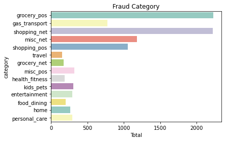
print(fullset['is_fraud'].value_counts())
	#visual the imbalanced data using charts
	fig= plt.figure(figsize=(10,5) )
	fig.add_subplot(1,2,1)
	explode = [0, 0.5]
	#labels = ['Fraud', 'Non-Fraud']
	a= fullset["is_fraud"].value_counts(normalize=True).plot.pie(explode=explode, autopct='%1.1f%%')
	fig.add_subplot(1,2,2)
	churnchart=sns.countplot(x=fullset["is_fraud"])
	plt.tight_layout()
	plt.show()
	0    1842743
	1       9651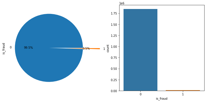
We want to check the distribution of our data using the histogram.
p = fullset.hist(figsize = (15,15))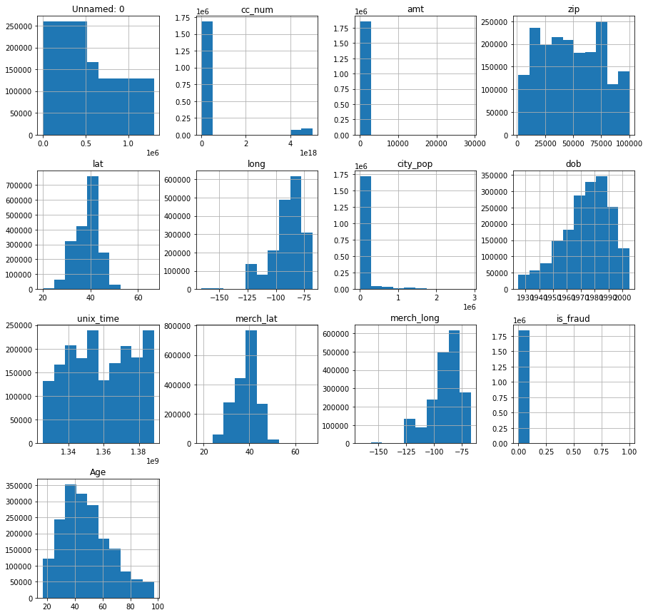
#apply label encoder to the dataset and put in the new dataset
newset = fullset.apply(LabelEncoder().fit_transform)

#plot correlation matrix
fig, ax = plt.subplots(figsize=(25,10))
sns.heatmap(newset.corr(), annot = True, ax=ax, cmap = 'Blues')
plt.title("DataCorrelation")
plt.show()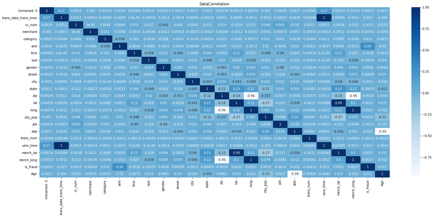
dropvar = ['is_fraud','Unnamed: 0', 'first', 'last', 'dob', 'trans_date_trans_time','trans_num', 'merch_lat', 'merch_long']
#create our dependent variables
x = newset.drop(dropvar, axis=1).copy()

#independent variable
y = newset['is_fraud'].copy()
Random Under Sampler
Undersampling is a technique to balance uneven datasets by keeping all of the data in the minority class and decreasing the size of the majority class. It is one of several techniques data scientists can use to extract more accurate information from originally imbalanced datasets.
Since our dataset is highly imbalance, we keep all the data of fraud class and decrease the samples from the non-fraud class.
#import library for random under sampler
import imblearn
from imblearn.under_sampling import RandomUnderSampler
import collections
from collections import Counter

#calling the method and fit it with x and y data
unSampler = RandomUnderSampler(random_state=42, replacement=True)
xund, yund = unSampler.fit_resample(x,y)

print('original dataset shape:', Counter(y))
print('resample dataset shape', Counter(yund))
	original dataset shape: Counter({0: 1842743, 1: 9651})
	resample dataset shape Counter({0: 9651, 1: 9651})
#visual the balanced data using bar chart
underfraud = pd.DataFrame(yund)
sns.countplot(x = 'is_fraud', data = underfraud)
plt.show()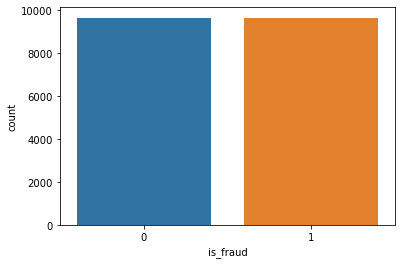
We will scale our data and perform PCA to reduce the dimensionality.
#scaling the data
mmscale = MinMaxScaler()
#transform the values
X_scaled = mmscale.fit_transform(xund)
from sklearn.decomposition import PCA
pca_15 = PCA(n_components = 15, random_state=2020)
pca_15.fit(X_scaled)
X_pca_15 = pca_15.transform(X_scaled)
#create following plot

plt.plot(np.cumsum(pca_15.explained_variance_ratio_))
plt.xlabel('Number of components')
plt.ylabel('Explained variance')
plt.savefig('elbow_plot.png', dpi= 100)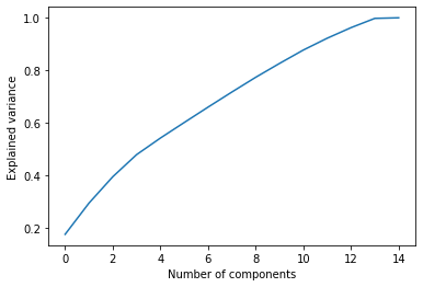
Function for metrix evaluation
score= []

#plot confusion matrixfrom sklearn.metrics import ConfusionMatrixDisplay, accuracy_score
from sklearn.metrics import log_loss, confusion_matrix, roc_auc_score, roc_curve

#plot the confusion matrix
def cm(algo): #it need the model variable after fitting the data
    disp = ConfusionMatrixDisplay(confusion_matrix=confusion_matrix(ytest, algo.predict(xtest)),
                           display_labels=algo.classes_)
    disp.plot()
    plt.show()

#print metrix score
#function to print metrics score
def prints(cmatrix, acctest, acctrain, overfit, logtest, logtrain, precision1,
                  precision0, recall1, recall0, f1, roctest, roctrain):
    print("Confusion Matrix Accuracy Score = {:.2f}%\n".format(cmatrix))
    print("Accuracy Score: Training -> {:.2f}% Testing -> {:.2f}%\n".format(acctrain, acctest))
    print("Overfitting : {:.2f}%".format(overfit))
    print("Log Loss Training-> {} Testing -> {}\n".format(logtrain, logtest))
    print('Precision class 1: {:.2f}%\nPrecision class 0: {:.2f}%'.format(precision1, precision0))
    print('Recall class 1: {:.2f}%\nRecall class 0: {:.2f}%'.format(recall1, recall0))
    print('F1: {:.2f}%'.format(f1))
    print('ROC AUC Training-> {:.2f}% Testing-> {:.2f}%'.format(roctrain, roctest))

#function add metrics score to list
def insertlist(name, cmatrix, acctest, acctrain,overfit, logtest, logtrain, precision1,
					precision0, recall1, recall0, f1, roctest, roctrain):
	score.append([name, cmatrix, acctest, acctrain,overfit, logtest, logtrain, precision1,
					precision0, recall1, recall0, f1, roctest, roctrain])

# Plot Roc Curve
def auc_plot(algo):
	#create AUC curve
	test_prob = algo.predict_proba(xtest)[::,1]
	train_prob = algo.predict_proba(xtrain)[::,1]
	roctest = roc_auc_score(ytest, test_prob)
	roctrain = roc_auc_score(ytrain, train_prob)

	fpr_test, tpr_test, _ = roc_curve(ytest,  test_prob)
	fpr_train, tpr_train, _ = roc_curve(ytrain,  train_prob)
	plt.title("Area Under Curve")
	plt.plot(fpr_test,tpr_test,label="AUC Test="+str(roctest))
	plt.plot(fpr_train,tpr_train,label="AUC Train="+str(roctrain))
	plt.ylabel('True Positive Rate')
	plt.xlabel('False Positive Rate')
	plt.legend(loc=4)
	plt.grid(True)
	plt.show()

#metrix function
def scr(algo, name): #algo = model, name = string of the model name
	predtest = algo.predict(xtest)
	predtrain = algo.predict(xtrain)

	#confussion matrix percentage
	tn, fp, fn, tp = confusion_matrix(ytest, predtest).ravel()
	tst = ytest.count()
	cmatrix = ((tn + tp)/tst)*100

	#accuracy score
	acctest = (accuracy_score(ytest, predtest))*100
	acctrain = (accuracy_score(ytrain, predtrain))*100
	overfit = acctrain - acctest

	#log loss
	logtest = log_loss(ytest,predtest)
	logtrain = log_loss(ytrain,predtrain)

	#classification report
	precision1 = (tp / (tp+fp))*100
	precision0 = (tn/(tn+fn))*100
	recall1 = (tp/(tp+fn))*100
	recall0 = (tn/(tn+fp))*100
	f1 = 2*(precision1 * recall1)/(precision1 + recall1)

	#roc auc score
	test_prob = algo.predict_proba(xtest)[::,1]
	train_prob = algo.predict_proba(xtrain)[::,1]
	roctest = (roc_auc_score(ytest, test_prob))*100
	roctrain = (roc_auc_score(ytrain, train_prob))*100

	insertlist(name, cmatrix, acctest, acctrain, overfit, logtest, logtrain, precision1,
				precision0, recall1, recall0, f1, roctest, roctrain)
	#print metrics score
	return prints(cmatrix, acctest, acctrain, overfit, logtest, logtrain, precision1,
					precision0, recall1, recall0, f1, roctest, roctrain)
xtrain, xtest, ytrain, ytest = train_test_split(x_pca, yund, test_size=0.3, random_state=42)Model 1 - Support Vector Machine
from sklearn.svm import SVC

#build SVM classification
SVM1 = SVC(random_state = 42, probability=True)
SVM1.fit(xtrain, ytrain)
scr(SVM1, 'SVM1')
cm(SVM1)
auc_plot(SVM1)

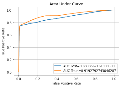
	Confusion Matrix Accuracy Score = 86.22%

	Accuracy Score: Training -> 86.94% Testing -> 86.22%

	Overfitting : 0.72%
	Log Loss Training-> 4.511955968344787 Testing -> 4.759453002690722

	Precision class 1: 97.25%
	Precision class 0: 79.36%
	Recall class 1: 74.55%
	Recall class 0: 97.89%
	F1: 84.40%
	ROC AUC Training-> 91.93% Testing-> 88.39%
kfold = StratifiedKFold(n_splits=10, shuffle=True, random_state=42)
param_grid = [
	{
		'C': [1, 10, 15, 20, 25, 30],
		'gamma': ['scale', 0.001, 0.01],
		'kernel': ['rbf','linear','sigmoid']
	},
]

#tuning the model using gridsearchCV and stratifiedkfold
optimal_param = GridSearchCV(
	SVC(), param_grid, cv=kfold, scoring='accuracy', verbose = 2)
	#fitting the tuned model with training dataset
optimal_param.fit(xtrain, ytrain)

#print the best parameter
print(optimal_param.best_params_)

	{'C': 15, 'gamma': 'scale', 'kernel': 'rbf'}
#build the model with hyperparameter tuning
optimal_param = SVC(random_state = 42, probability=True, C=20, gamma='scale', kernel='rbf')
optimal_param.fit(xtrain,ytrain)
#print metrics score
scr(optimal_param, 'SVM_tuned')
#plot confusion matrix for the tuned model
cm(optimal_param)
#plot the learning curve
auc_plot(optimal_param)
Confusion Matrix Accuracy Score = 87.65%
Accuracy Score: Training -> 93.07% Testing -> 87.65%
Overfitting : 5.42%
Log Loss Training-> 2.392745485940981 Testing -> 4.26443851713289
Precision class 1: 93.15%
Precision class 0: 83.39%
Recall class 1: 81.28%
Recall class 0: 94.02%
F1: 86.82%
ROC AUC Training-> 97.61% Testing-> 93.11%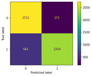
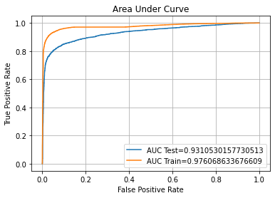
After Tuning Accuracy score is 87.71%
However, model is slightly overfit after hypertuning.
Model 2 - Logistic Regression
#create logistic regression model
logreg = LogisticRegression()
#fitting the model with training dataset
logreg.fit(xtrain, ytrain)
scr(logreg, 'Logreg')
cm(logreg)
auc_plot(logreg)
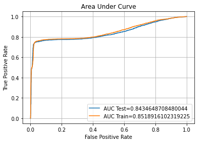
	Confusion Matrix Accuracy Score = 84.63%

	Accuracy Score: Training -> 85.06% Testing -> 84.63%

	Overfitting : 0.43%
	Log Loss Training-> 5.15872999693614 Testing -> 5.308178710927689

	Precision class 1: 92.04%
	Precision class 0: 79.44%
	Recall class 1: 75.83%
	Recall class 0: 93.44%
	F1: 83.15%
	ROC AUC Training-> 85.19% Testing-> 84.35%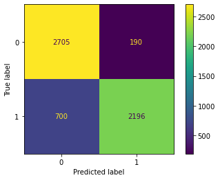
log_param = [
	{
		'C': [0.01, 0.1, 1.0, 10, 100],
		'penalty': ['l2'],
		'solver': ['newton-cg', 'sag','saga']
	},
]

#tuned the model using gridsearch and kfold
opt_log = GridSearchCV(LogisticRegression(), param_grid = log_param, scoring='accuracy', cv=kfold, verbose = 2)

#fit the tuned model with training dataset
opt_log.fit(xtrain, ytrain)
print(opt_log.best_params_)
	{'C': 0.01, 'penalty': 'l2', 'solver': 'newton-cg'}
opt_log = LogisticRegression(random_state = 42, C=0.012, penalty = 'l2', solver = 'sag' )
opt_log.fit(xtrain, ytrain)
scr(opt_log, 'logreg_tuned')
cm(opt_log)
auc_plot(opt_log)
Confusion Matrix Accuracy Score = 85.17%
Accuracy Score: Training -> 85.54% Testing -> 85.17%
Overfitting : 0.37%
Log Loss Training-> 4.9951177071719135 Testing -> 5.123281655199142
Precision class 1: 93.81%
Precision class 0: 79.37%
Recall class 1: 75.31%
Recall class 0: 95.03%
F1: 83.55%
ROC AUC Training-> 84.62% Testing-> 83.81%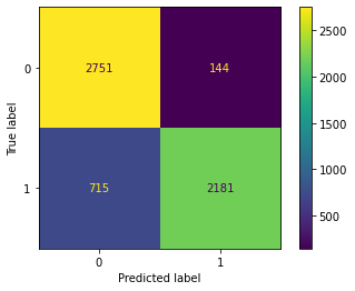

After Tuning Accuracy = 85.17%
Overfitting is reduced as well.
Model 3 - Random Forest
from sklearn.ensemble import RandomForestClassifier
RF = RandomForestClassifier()
#fit the model with training dataset
RF.fit(xtrain, ytrain)
scr(RF, 'RF')
cm(RF)
auc_plot(RF)
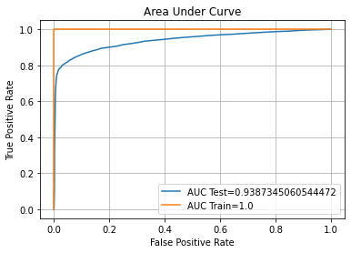
	Confusion Matrix Accuracy Score = 88.57%

	Accuracy Score: Training -> 100.00% Testing -> 88.57%

	Overfitting : 11.43%
	Log Loss Training-> 9.992007221626413e-16 Testing -> 3.948323732826286

	Precision class 1: 96.23%
	Precision class 0: 83.08%
	Recall class 1: 80.28%
	Recall class 0: 96.86%
	F1: 87.54%
	ROC AUC Training-> 100.00% Testing-> 93.87%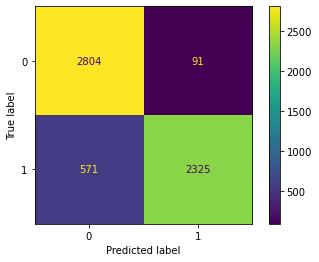
# Number of trees in random forest
n_estimators = [int(x) for x in np.linspace(start = 100, stop = 1000, num = 50)]
# Number of features to consider at every split
max_features = ['auto', 'sqrt']
# Maximum number of levels in tree
max_depth = [int(x) for x in np.linspace(1, 100, num = 10)]
max_depth.append(None)
# Minimum number of samples required to split a node
min_samples_split = [2, 5, 10, 15, 100]
# Minimum number of samples required at each leaf node
min_samples_leaf = [1, 2, 5, 10, 50, 100]
# Method of selecting samples for training each tree
bootstrap = [True, False]

random_grid = {'n_estimators': n_estimators,
				'max_features': max_features,
				'max_depth': max_depth,
				'min_samples_split': min_samples_split,
				'min_samples_leaf': min_samples_leaf,
				'bootstrap': bootstrap}

#implement parameter tuning using randomized search cv and kfold
opt_RF = RandomizedSearchCV(estimator = RF, param_distributions = random_grid, n_iter = 100, cv = kfold, verbose=2, random_state=42, n_jobs = -1)
#fit the model with training dataset
opt_RF.fit(xtrain, ytrain)
print(opt_RF.best_params_) #best parameter tuning result
	{'n_estimators': 853, 'min_samples_split': 5, 'min_samples_leaf': 1, 'max_features': 'sqrt', 'max_depth': 78, 'bootstrap': False}
#build the model with hyperparameter tuning
opt_RF = RandomForestClassifier(n_estimators= 600, min_samples_split= 5, min_samples_leaf= 2,max_features= 'auto',max_depth= 6)
opt_RF.fit(xtrain, ytrain)
scr(opt_RF, 'RF_tuned')
cm(opt_RF)
auc_plot(opt_RF)
Confusion Matrix Accuracy Score = 85.74%
Accuracy Score: Training -> 86.15% Testing -> 85.74%
Overfitting : 0.42%
Log Loss Training-> 4.782934449404927 Testing -> 4.926456581166755
Precision class 1: 95.55%
Precision class 0: 79.40%
Recall class 1: 74.97%
Recall class 0: 96.51%
F1: 84.02%
ROC AUC Training-> 90.47% Testing-> 87.91%Model 4 - Decision Tree
#import the library
from sklearn.tree import DecisionTreeClassifier
#create the model
decTree = DecisionTreeClassifier()
#fit the model with training data
decTree.fit(xtrain, ytrain)
scr(decTree, 'decTree')
cm(decTree)
auc_plot(decTree)
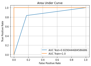
	Confusion Matrix Accuracy Score = 82.90%

	Accuracy Score: Training -> 100.00% Testing -> 82.90%

	Overfitting : 17.10%
	Log Loss Training-> 9.992007221626413e-16 Testing -> 5.904643831404563

	Precision class 1: 82.68%
	Precision class 0: 83.13%
	Recall class 1: 83.25%
	Recall class 0: 82.56%
	F1: 82.97%
	ROC AUC Training-> 100.00% Testing-> 82.90%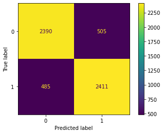
#parameter variables
criterion = ['gini', 'entropy']
max_depth = [3,6,9]
min_samples_split = [3,6,9]
min_samples_leaf = [2,4,8]

#put the variables to dict
random_tree = {'criterion': criterion,
				'max_depth': max_depth,
				'min_samples_split': min_samples_split,
				'min_samples_leaf': min_samples_leaf}

#implement hyperparameter tuning to the model
opt_decTree = DecisionTreeClassifier(min_samples_split = 7, min_samples_leaf = 40, max_depth = 5)
#fit the model with training dataset
opt_decTree.fit(xtrain, ytrain)
#fit the model with training dataset
opt_decTree.fit(xtrain, ytrain)
print(opt_decTree.best_params_)
	{'min_samples_split': 9, 'min_samples_leaf': 8, 'max_depth': 9, 'criterion': 'gini'}

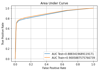
	Confusion Matrix Accuracy Score = 85.81%

	Accuracy Score: Training -> 89.08% Testing -> 85.81%

	Overfitting : 3.27%
	Log Loss Training-> 3.773181988317355 Testing -> 4.90261131447784

	Precision class 1: 92.43%
	Precision class 0: 80.97%
	Recall class 1: 78.00%
	Recall class 0: 93.61%
	F1: 84.61%
	ROC AUC Training-> 94.47% Testing-> 89.99%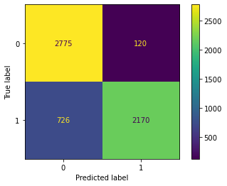
Model 5 - K-Nearest Neighbor
from sklearn.neighbors import KNeighborsClassifier

#build the model
neigh = KNeighborsClassifier(n_neighbors=3)
#fit the model with training dataset
neigh.fit(xtrain, ytrain)
scr(neigh, 'KNN')
cm(neigh)
auc_plot(neigh)
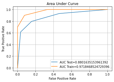
	Confusion Matrix Accuracy Score = 82.01%

	Accuracy Score: Training -> 91.15% Testing -> 82.01%

	Overfitting : 9.14%
	Log Loss Training-> 3.0574194329192323 Testing -> 6.214775759201414

	Precision class 1: 83.61%
	Precision class 0: 80.55%
	Recall class 1: 79.63%
	Recall class 0: 84.39%
	F1: 81.57%
	ROC AUC Training-> 97.18% Testing-> 88.02%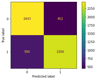
tuning_params = {
	'n_neighbors' : [71,75,77,83], #from the plot above
	"leaf_size":[5,10,20,30],
	"p":[1,2]
}

#implement hyperparameter tuning to the model
opt_knn = GridSearchCV(neigh, param_grid = tuning_params, cv = kfold, verbose = 1, n_jobs = -1)
#fit the model with training dataset
opt_knn.fit(xtrain, ytrain)
print(opt_knn.best_params_)
scr(opt_knn, 'knn_tuned')
cm(opt_knn)
auc_plot(opt_knn)
	{'leaf_size': 5, 'n_neighbors': 83, 'p': 1}

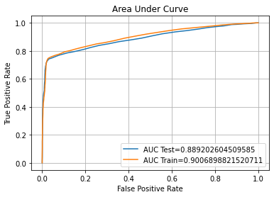
	Confusion Matrix Accuracy Score = 85.24%

	Accuracy Score: Training -> 85.66% Testing -> 85.24%

	Overfitting : 0.43%
	Log Loss Training-> 4.951649723316238 Testing -> 5.099414020217411

	Precision class 1: 96.96%
	Precision class 0: 78.19%
	Recall class 1: 72.76%
	Recall class 0: 97.72%
	F1: 83.13%
	ROC AUC Training-> 90.07% Testing-> 88.92%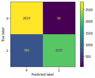
Model 6 - Artificial Neural Network
Xtrain, xrem, Ytrain, yrem = train_test_split(xtrain,ytrain, train_size=0.6)
xvalid, xtest, yvalid, ytest = train_test_split(xrem,yrem, test_size=0.5)
#build the model
ann=keras.Sequential([keras.layers.Dense(20,input_shape=(14,),activation='relu'),
                       keras.layers.Dense(1,activation='sigmoid'),])
ann.compile(optimizer='adam',loss='binary_crossentropy',metrics=['accuracy', tf.keras.metrics.AUC()])
#train the model
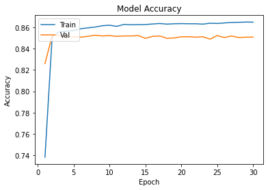
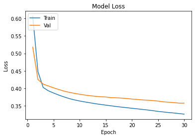
history=ann.fit(Xtrain,Ytrain,epochs=30,validation_data=(xvalid,yvalid))
plot_learningCurve(history,30)
testeval1 = ann.evaluate(xtest, ytest)
traineval1 = ann.evaluate(xvalid, yvalid)
yprediction=ann.predict(xtest)
ypred=[]
for element in yprediction:
    if element>0.5:
        ypred.append(1)
    else:
        ypred.append(0)

#plot confusion matrix
cmt =tf.math.confusion_matrix(labels=ytest,predictions=ypred)
plt.figure(figsize=(7,5))
sns.heatmap(cmt,annot=True,fmt='d')
plt.xlabel('predicted')
plt.ylabel('actual')
#print the metrics score
calc(ann, 'ann', testeval1, traineval1, cmt)

	Confusion Matrix Accuracy Score = 86.24%

	Accuracy Score: Training -> 85.09% Testing -> 86.24%

	Overfitting : -1.15%
	Log Loss Training-> 0.35751211643218994 Testing -> 0.3230932652950287

	Precision class 1: 96.95%
	Precision class 0: 79.77%
	Recall class 1: 74.30%
	Recall class 0: 97.75%
	F1: 84.13%
	ROC AUC Training-> 90.58% Testing-> 91.87%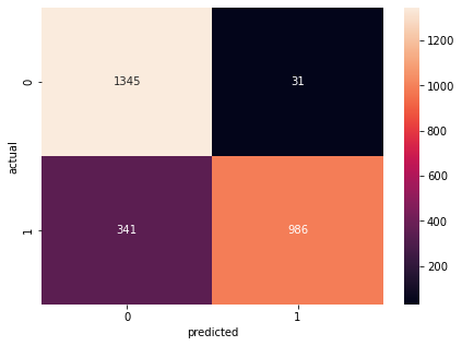
opt_ann=create_my_model1()
#train the model
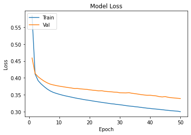
history=opt_ann.fit(Xtrain,Ytrain,epochs=50,batch_size = 15,validation_data=(xvalid,yvalid))
plot_learningCurve(history,50)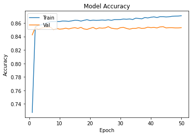
calc(opt_ann, 'ann_tuned', testeval, traineval, cm1)
cm1 =tf.math.confusion_matrix(labels=ytest,predictions=ypred1)
plt.figure(figsize=(7,5))
sns.heatmap(cm1,annot=True,fmt='d')
plt.xlabel('predicted')
plt.ylabel('actual')
	Confusion Matrix Accuracy Score = 86.72%

	Accuracy Score: Training -> 85.09% Testing -> 86.24%

	Overfitting : -1.15%
	Log Loss Training-> 0.35751211643218994 Testing -> 0.3230932652950287

	Precision class 1: 96.36%
	Precision class 0: 80.65%
	Recall class 1: 75.81%
	Recall class 0: 97.24%
	F1: 84.86%
	ROC AUC Training-> 90.58% Testing-> 91.87%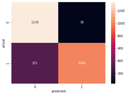
Model 7 - Convolutional Neural Networks
epochs=20
cnn=Sequential()
cnn.add(Conv1D(32,2, activation='relu',input_shape=Xtrain[0].shape))
cnn.add(BatchNormalization())
cnn.add(Dropout(0.2))

cnn.add(Conv1D(64,2, activation='relu'))
cnn.add(BatchNormalization())
cnn.add(Dropout(0.5))

cnn.add(Flatten())
cnn.add(Dense(64,activation='relu'))
cnn.add(Dropout(0.5))

cnn.add(Dense(1,activation='sigmoid'))
cnn.compile(optimizer=Adam(learning_rate=0.0001),loss='binary_crossentropy',metrics=['accuracy',
	tf.keras.metrics.AUC()])

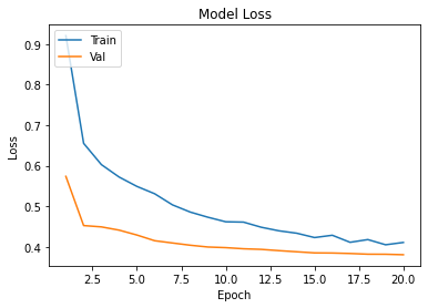
	history=cnn.fit(Xtrain,Ytrain,epochs=epochs,validation_data=(xvalid,yvalid))
plot_learningCurve(history,epochs)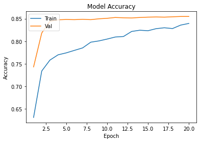
cntesteval = cnn.evaluate(xtest, ytest)
cntraineval = cnn.evaluate(Xtrain,Ytrain)
cnypredict=cnn.predict(xtest)
ypred2=[]
for element in cnypredict:
    if element>0.5:
        ypred2.append(1)
    else:
        ypred2.append(0)

cm2 =tf.math.confusion_matrix(labels=ytest,predictions=ypred2)
plt.figure(figsize=(7,5))
sns.heatmap(cm2,annot=True,fmt='d')
plt.xlabel('predicted')
plt.ylabel('actual')

calc(cnn, 'cnn', cntesteval, cntraineval, cm2)
	Confusion Matrix Accuracy Score = 86.68%

	Accuracy Score: Training -> 86.53% Testing -> 86.68%

	Overfitting : -0.15%
	Log Loss Training-> 0.35620877146720886 Testing -> 0.3592900037765503

	Precision class 1: 96.99%
	Precision class 0: 80.35%
	Recall class 1: 75.21%
	Recall class 0: 97.75%
	F1: 84.72%
	ROC AUC Training-> 90.13% Testing-> 89.15%
epochs=50
cnnmax=Sequential()
cnnmax.add(Conv1D(32,2, activation='relu',input_shape=Xtrain[0].shape))
cnnmax.add(BatchNormalization())
cnnmax.add(MaxPool1D(2))
cnnmax.add(Dropout(0.2))

cnnmax.add(Conv1D(64,2, activation='relu'))
cnnmax.add(BatchNormalization())
cnnmax.add(MaxPool1D(2))
cnnmax.add(Dropout(0.5))

cnnmax.add(Flatten())
cnnmax.add(Dense(64,activation='relu'))
cnnmax.add(Dropout(0.5))

cnnmax.add(Dense(1,activation='sigmoid'))

cnnmax.compile(optimizer=Adam(learning_rate=0.0001),loss='binary_crossentropy',metrics=['accuracy',
	tf.keras.metrics.AUC()])
history2=cnnmax.fit(Xtrain,Ytrain,epochs=100,validation_data=(xvalid,yvalid))

plot_learningCurve(history2,100)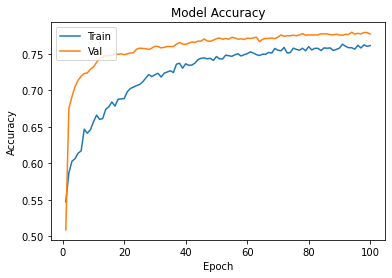
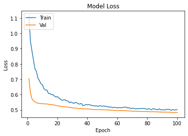
calc(cnn, 'cnn_tuned', maxtesteval, maxtraineval, cm3)
#plot confusion matrix
cm3 =tf.math.confusion_matrix(labels=ytest,predictions=ypred3)
plt.figure(figsize=(7,5))
sns.heatmap(cm3,annot=True,fmt='d')
plt.xlabel('predicted')
plt.ylabel('actual')
	Confusion Matrix Accuracy Score = 77.28%

	Accuracy Score: Training -> 78.63% Testing -> 77.28%

	Overfitting : 1.35%
	Log Loss Training-> 0.46808817982673645 Testing -> 0.48547038435935974

	Precision class 1: 89.22%
	Precision class 0: 71.24%
	Recall class 1: 61.12%
	Recall class 0: 92.88%
	F1: 72.54%
	ROC AUC Training-> 85.53% Testing-> 83.94%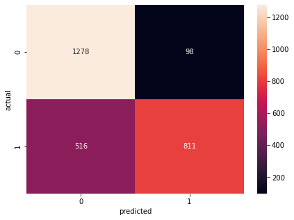
Conclusion
scoring = pd.DataFrame(score, columns = ['algo','c_matrix','acc_test','acc_train','overfit', 'loss_test',
'loss_train', 'prec1', 'prec0', 'recall1','recall0', 'F1', 'roctest', 'roctrain'])| algo | c_matrix | acc_test | acc_train | overfit | loss_test | loss_train | prec1 | prec0 | recall1 | recall0 | F1 | roctest | roctrain | |
|---|---|---|---|---|---|---|---|---|---|---|---|---|---|---|
| 0 | SVM1 | 86.219997 | 86.219997 | 86.936570 | 0.716574 | 4.759453 | 4.511956e+00 | 97.252252 | 79.361523 | 74.551105 | 97.892919 | 84.401876 | 88.385672 | 91.927927 |
| 1 | SVM_tuned | 87.653255 | 87.653255 | 93.072311 | 5.419056 | 4.264439 | 2.392745e+00 | 93.153937 | 83.394608 | 81.284530 | 94.024180 | 86.815416 | 93.105302 | 97.606863 |
| 2 | Logreg | 84.631324 | 84.631324 | 85.064022 | 0.432697 | 5.308179 | 5.158730e+00 | 92.036882 | 79.441997 | 75.828729 | 93.436960 | 83.150322 | 84.346487 | 85.189161 |
| 3 | logreg_tuned | 85.166638 | 85.166638 | 85.537710 | 0.371072 | 5.123282 | 4.995118e+00 | 93.806452 | 79.371033 | 75.310773 | 95.025907 | 83.547213 | 83.811320 | 84.624693 |
| 4 | RF | 88.568468 | 88.568468 | 100.000000 | 11.431532 | 3.948324 | 9.992007e-16 | 96.233444 | 83.081481 | 80.283149 | 96.856649 | 87.537651 | 93.873451 | 100.000000 |
| 5 | RF_tuned | 88.982905 | 88.982905 | 100.000000 | 11.017095 | 3.805185 | 9.992007e-16 | 95.597738 | 84.042232 | 81.733425 | 96.234888 | 88.123604 | 94.519837 | 100.000000 |
| 6 | RF_tuned | 85.736488 | 85.736488 | 86.152024 | 0.415537 | 4.926457 | 4.782934e+00 | 95.554577 | 79.397556 | 74.965470 | 96.511226 | 84.017028 | 87.914007 | 90.470434 |
| 7 | decTree | 82.904507 | 82.904507 | 100.000000 | 17.095493 | 5.904644 | 9.992007e-16 | 82.681756 | 83.130435 | 83.252762 | 82.556131 | 82.966277 | 82.904447 | 100.000000 |
| 8 | decTree_tuned | 85.805560 | 85.805560 | 89.075568 | 3.270008 | 4.902611 | 3.773182e+00 | 92.430442 | 80.968031 | 78.004144 | 93.609672 | 84.606742 | 89.989355 | 94.472079 |
| 9 | decTree_tuned | 85.391124 | 85.391124 | 86.129820 | 0.738696 | 5.045744 | 4.790606e+00 | 94.759825 | 79.263068 | 74.930939 | 95.854922 | 83.686849 | 88.834197 | 90.058876 |
| 10 | KNN | 82.006562 | 82.006562 | 91.147954 | 9.141392 | 6.214776 | 3.057419e+00 | 83.611313 | 80.547313 | 79.627072 | 84.386874 | 81.570570 | 88.016352 | 97.184685 |
| 11 | knn_tuned | 85.287515 | 85.287515 | 85.663533 | 0.376018 | 5.081522 | 4.951650e+00 | 96.794872 | 78.319933 | 72.997238 | 97.582038 | 83.228346 | 89.064966 | 90.235731 |
| 12 | knn_tuned | 85.235711 | 85.235711 | 85.663533 | 0.427823 | 5.099414 | 4.951650e+00 | 96.962724 | 78.192371 | 72.755525 | 97.720207 | 83.132768 | 88.920260 | 90.068988 |
| 13 | ann | 86.237514 | 86.237514 | 85.085124 | -1.152390 | 0.323093 | 3.575121e-01 | 96.951819 | 79.774614 | 74.302939 | 97.747093 | 84.129693 | 91.869640 | 90.576106 |
| 14 | ann_tuned | 86.718461 | 86.237514 | 85.085124 | -1.152390 | 0.323093 | 3.575121e-01 | 96.360153 | 80.650995 | 75.810098 | 97.238372 | 84.858709 | 91.869640 | 90.576106 |
| 15 | cnn | 86.681465 | 86.681467 | 86.528498 | -0.152969 | 0.359290 | 3.562088e-01 | 96.987366 | 80.346476 | 75.207234 | 97.747093 | 84.719864 | 89.148206 | 90.132415 |
| 16 | cnn_tuned | 77.284499 | 77.284497 | 78.633112 | 1.348615 | 0.485470 | 4.680882e-01 | 89.218922 | 71.237458 | 61.115298 | 92.877907 | 72.540250 | 83.936465 | 85.533202 |
Hyperparameter tuning, K-Fold cross-validation and validation curves are applied to cope with the overfitting problem and to improve the accuracy. As a result, the overfit in Random Forest and Decision Tree are dropped by almost 10% by changing some of the parameters, and the accuracy score is also increased for Decision Tree from 82.90% to 85.39%.
For future benefits, we selected three algorithms with the lowest percentage of overfitting as they will generalise well to new data. If the model can generalise the data well, it also could perform the classification or prediction task that was intended for. Consequently, we picked Logistic Regression, Decision Trees and CNN as our final algorithm for the credit card fraud detection problem.